Wed Oct 28, 2026 Lecture (L25) Stewart Section 4.4 Graphing
 Watch on YouTube →
Overview
The lecture finishes Section 4.3 with the second derivative test for local extrema, then develops a four-step graphing strategy for Stewart Section 4.4: analyze the function, its first derivative, and its second derivative before sketching. A worked example, f(x) = x/√(x² + 9), shows how domain, intercepts, odd symmetry, horizontal asymptotes, monotonicity, and concavity combine to determine a graph; follow-up rational-function examples illustrate how small formula changes alter graph features.
Key takeaways
- At a critical point c with f′(c) = 0, the sign of f″(c) identifies a local minimum when positive and a local maximum when negative; f″(c) = 0 makes this test inconclusive.
- A reliable graphing workflow is to establish domain and basic features first, use f′ for monotonicity and extrema, use f″ for concavity, and then combine the results into a sketch.
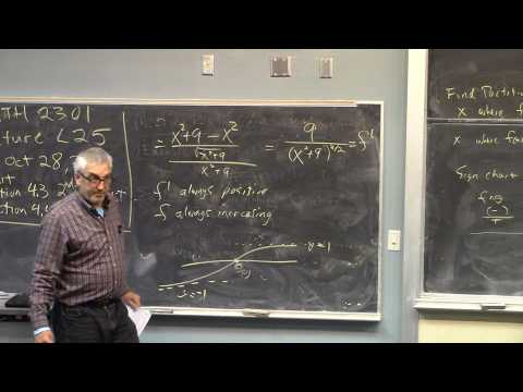
- For f(x) = x/√(x² + 9), the derivative 9/(x² + 9)^(3/2) is always positive, while the limits at positive and negative infinity are 1 and −1.
- The second derivative of x/√(x² + 9) is −27x/(x² + 9)^(5/2), so the graph changes from concave up to concave down at its inflection point (0, 0).
- Even and odd symmetry can reduce graphing work: even functions mirror across the y-axis, while odd functions have origin symmetry.
- For rational functions, denominator zeros can create vertical asymptotes, while numerator zeros create x-intercepts; comparing examples such as x² + 25 and x² − 25 makes these effects clear.
Chapters
- The test applies at a critical point c when f′(c) = 0 and f is continuous near c.
- If f″(c) > 0, the graph is concave up and c is a local minimum; if f″(c) < 0, it is concave down and c is a local maximum.
- If both f′(c) and f″(c) equal zero, the test is inconclusive rather than evidence that no extremum exists.
- For y = x², y′(0) = 0 and y″(0) = 2, so the test identifies a minimum at x = 0.
- For y = −x², y′(0) = 0 and y″(0) = −2, identifying a maximum at x = 0.
- For y = x³ and y = x⁴, both derivatives vanish at zero, so the test cannot distinguish the cubic's lack of an extremum from the quartic's minimum.
- Step 1 examines the function using familiar precalculus features: domain, intercepts, vertical asymptotes, symmetry, periodicity, and end behavior.
- Step 2 uses f′ to locate increasing and decreasing intervals and local extrema; Step 3 uses f″ to determine concavity.
- Step 4 combines those findings into a sketch, and difficult steps can be postponed while other information is gathered.
- The instructor recommends completing at least four full graphing problems, noting that practice can reduce the time from about an hour to around 10 minutes.
- The assigned problems cover third- and fourth-degree polynomials, products involving powers and exponentials, and rational functions.
- Reading Section 4.4 examples and attempting homework before recitation can prepare students for quiz questions modeled on book examples.
- The denominator √(x² + 9) is always positive because x² + 9 ≥ 9, so the function is continuous for every real x and has no vertical asymptotes.
- Setting x = 0 gives the y-intercept (0, 0); the numerator is zero only at x = 0, so this is also the sole x-intercept.
- The denominator is positive everywhere, so the sign of f matches the sign of x: negative to the left of zero and positive to the right.
- Replacing x with −x gives f(−x) = −f(x), establishing odd symmetry and an origin-centered, 180-degree rotational relationship between the two sides.
- Dividing by the dominant growth in √(x² + 9) shows that f(x) approaches 1 as x approaches positive infinity.
- At negative infinity, f(x) approaches −1, giving horizontal asymptotes y = 1 on the right and y = −1 on the left.
- Applying the quotient rule and simplifying gives f′(x) = 9/(x² + 9)^(3/2).
- Both the numerator and denominator of f′ are positive for every real x, so f is strictly increasing throughout its domain.
- Together with (0, 0) and the asymptotes y = −1 and y = 1, this determines the graph's overall rising shape.
- Differentiating again gives f″(x) = −27x/(x² + 9)^(5/2).
- The denominator stays positive, while the numerator changes sign at x = 0: f″ is positive for x < 0 and negative for x > 0.
- The graph is concave up on the left and concave down on the right, with an inflection point at (0, 0) and no local extrema.
- The next example is described as an even rational function with domain all real numbers, y-intercept (0, 4), no x-intercepts, and horizontal asymptote y = 0.
- Because it is always positive and symmetric about the y-axis, its graph stays above the x-axis and mirrors across that axis.
- Its derivative is positive for x < 0 and negative for x > 0, confirming a maximum at x = 0; the second derivative changes sign at x = ±5/√3.
- Changing a denominator from x² + 25 to x² − 25 creates denominator zeros at x = −5 and x = 5, producing two vertical asymptotes.
- With a numerator that never vanishes, the graph has no x-intercepts and never crosses the x-axis.
- Changing the numerator to 100x while retaining x² + 25 creates an x-intercept at zero, illustrating how small formula changes affect the graph.
Transcript excerpt
0:02 Um this is Wednesday. [snorts] This is lecture 25. We're discussing uh 4.4 today graphing. But I want to start with a a leftover topic from section 4.3. So that's meeting part one. So the second derivative test, [cough] excuse me, second derivative test. So this is a test for for local extreme
0:57 Excuse [cough] me. Test for local extrema. So remember our quest articulated last week. I wanted to come up with we we want to uh develop analytical tools so that we could by analyzing the formula for a function determine where the function had maxes and mins. things that are easy to see on a graph. We wanted to have analytical tools to detect these things from uh from from formulas for functions. So we we had last week the uh closed interval test. If you have a continuous function on a closed interval
1:47 um continuous and differentiable well it doesn't have to be differentiable everywhere. the functions guaranteed to have an absolute max and an absolute min on that interval. And you we found those maxes and mins by just making a list of the important x values where they had to occur. They had to occur either at the end points or at x values that are critical numbers. That was uh a partial fulfillment of our quest. U again we're we're be looking for tools that will find maxes and ms. And then uh was it Monday? I introduced the increasing decreasing test that um well let me just project this now. I guess we talked about this on Friday.
2:44 We we on on Friday we talked about the fact that we can determine um from the sign behavior of fprime where a function is uh where f is increasing or decreasing. So if fprime
This is the start of the transcript. Save this video free for the whole transcript, searchable and time-coded.
Related notes
Summary, takeaways, and chapters were generated by AI from the video's transcript and may contain errors. The video belongs to its creator, Barsamian's Math Videos.