More about concavity; introduction to optimization (Calc 1; Lecture 2-9; Fall 26)

Overview

The lecture connects concavity and derivative tests to curve sketching, then introduces optimization as the process of expressing a maximum or minimum as a single-variable function. Examples include estimating 2√4.2 as 4.1, sketching a cubic from derivative signs, classifying a product's critical point, and maximizing the area of a riverside rectangle with 400 feet of fencing.

Key takeaways

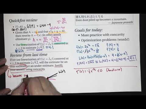
A constraint can eliminate a variable: x²y + y = 40 gives y = 40/(x² + 1), turning a = xy into a single-variable function.
For 2√x at x = 4, the tangent-line approximation is 4 + ½(x − 4); because the function is concave down for x > 0, its estimate of 2√4.2 = 4.1 is an overestimate.
A reliable rough sketch combines critical points and inflection candidates with the signs of f′ and f″ on every interval between them.
At a critical point, sampled derivative values farther away do not necessarily establish nearby behavior; for the product example, h″(2) = −3 supplies the valid local-maximum classification.
For a riverside rectangle using 400 feet of fencing, A(W) = 400W − 2W² is maximized at W = 100 feet and L = 200 feet, producing 20,000 square feet.

Chapters

0:00 Difference of Squares and Turning a Constraint into One Variable

Compute 77 × 83 mentally by writing the factors as 80 − 3 and 80 + 3, then applying (a − b)(a + b) = a² − b² to get 6,391.
For a = xy with x²y + y = 40, factor out y to obtain y = 40/(x² + 1), so a can be written as a function of x alone.
The constraint connects x and y; substituting it reduces a two-variable expression to the single variable required in Calc 1.

3:55 Linearizing 2√x at x = 4 to Estimate 2√4.2

Treat the linearization centered at x = 4 as the tangent-line approximation, using f(x) = 2√x and f′(x) = 1/√x.
At x = 4, f(4) = 4 and f′(4) = 1/2, giving L(x) = 4 + ½(x − 4).
Substituting x = 4.2 gives L(4.2) = 4.1, an estimate for 2√4.2.

7:18 Using Concavity to Determine the Direction of Linearization Error

For f(x) = 2√x, the second derivative is f″(x) = −½x^(−3/2), which is negative for x > 0.
Because the function is concave down near x = 4, its graph lies below the tangent line there.
The tangent-line estimate 4.1 for 2√4.2 is therefore an overestimate; concavity identifies the direction of error, not its exact size.

12:19 A Derivative-Sign Recipe for Rough Curve Sketches

A computer sketch can connect many plotted points; a calculus sketch instead identifies where f′ or f″ is zero or undefined and checks signs between those points.
The signs of f′ and f″ determine whether a curve is increasing or decreasing and concave up or down.
Plot the important points, determine the behavior on each interval, then connect the points with a curve that matches those signs.

17:48 Sketching x³ − 3x² − 9x + 15 from Critical Points and Concavity

For f(x) = x³ − 3x² − 9x + 15, f′ has zeros at x = −1 and 3, while f″ is zero at x = 1.
The key plotted points are (−1, 20), (1, 4), and (3, −12); x = −1 is a local maximum, x = 3 a local minimum, and x = 1 an inflection point.
The curve is increasing and concave down before −1, decreasing and concave down from −1 to 1, decreasing and concave up from 1 to 3, then increasing and concave up after 3.

26:08 Classifying a Product’s Critical Point with the Second Derivative Test

For h(x) = f(x)g(x), use h′ = f′g + fg′ and the supplied table to test x = 0, 1, 2, and 3; only h′(2) equals zero.
The table values at x = 1 and x = 3 cannot establish the first-derivative sign immediately around x = 2, so the first-derivative test is not justified from those samples alone.
Apply h″ = f″g + 2f′g′ + fg″; the table gives h″(2) = −3, so the second-derivative test classifies x = 2 as a local maximum.

35:29 Reading f′ and f″ Graphs to Analyze f on [−4, 2]

From the graph of f′, its local extrema at x = −3 and x = −1 mark zeros of f″; f′ increases between those points and decreases elsewhere.
Since f′ is above the axis from −4 to 1 and below it from 1 to 2, f increases on (−4, 1) and decreases on (1, 2), with a local maximum at x = 1.
The graph implies f″ is positive on (−3, −1) and negative on (−4, −3) and (−1, 2), giving inflection points at x = −3 and x = −1.

41:49 Optimization as a Single-Variable Critical-Point Problem

Optimization asks for a best outcome, often signaled by words such as maximum, minimum, most, or least.
Set up the problem by identifying the quantity to optimize, the variables that can change, and any constraint linking them; a diagram can help organize the relationships.
Translate the conditions into a function of one variable, find and classify critical points, then check that the result answers the question and has appropriate units.

45:58 Maximizing Riverside Rectangle Area with 400 Feet of Fencing

For a rectangle beside a river, one side needs no fence; if the fenced side is L and each perpendicular side is W, the constraint is L + 2W = 400.
Write L = 400 − 2W and substitute into A = LW to get A(W) = 400W − 2W².
Solving A′(W) = 400 − 4W = 0 gives W = 100 feet and L = 200 feet, for a maximum area of 20,000 square feet.

Summary, takeaways, and chapters were generated by AI from the video's transcript and may contain errors. The video belongs to its creator, Beard Meets Calculus.