ME2120 - Dynamics
 Watch on YouTube →
Overview
Ryan C. Cooper compares the nonlinear pendulum equation, θ̈ = −(g/L)sinθ, with its small-angle linearization, θ̈ = −(g/L)θ, using simulations to show how their predictions diverge at large angles and converge near 10°. He also outlines a 3D-printed spinning-top project, explains how to quantify differences in period, acceleration, and tension, and previews angular momentum.
Key takeaways
- The small-angle pendulum model replaces sinθ with θ, an approximation that becomes more accurate as the angle approaches zero.
- At 30°, the linear and nonlinear pendulum simulations remain close, while at 60° their periods and phases visibly diverge.
- At π radians, sinθ equals zero but the linear approximation θ does not, producing a dramatic failure of the linear model near the inverted equilibrium.
- A pendulum’s angular velocity converts to tangential speed through v = Lθ̇, and its tension can be calculated after solving for θ and θ̇.
- Model error should be defined and quantified, for example by comparing periods or acceleration amplitudes, because graph differences may be smaller than measurement resolution.
- Binder sessions do not retain project files, so students need to save their notebooks externally before ending a session.
Chapters
- The ideal pendulum model includes tension and gravity but no drag, friction, or damping, so its oscillations do not decay.
- The class compares a nonlinear swinging pendulum with a linearized, spring-like approximation.
- Cooper notes that increasing the initial angle lengthens the nonlinear pendulum’s period, motivating the question of when the small-angle model is adequate.
- The sine expansion begins sinθ = θ − θ³/3! + θ⁵/5!, while the cosine expansion begins cosθ = 1 − θ²/2 + θ⁴/4!.
- For θ much smaller than 1 radian, the leading approximations are sinθ ≈ θ and cosθ ≈ 1.
- Cooper emphasizes that engineering linearization often retains only the first terms, with angles expressed in radians.
- The upcoming case study asks students to design and 3D-print a spinning top, with the in-class competition moved to Monday the 16th to allow 12 days for design and printing.
- Students can visit the Innovation Shop for training and printing support; Cooper names Anthony and Joe as shop contacts.
- The minimum submission is one spinning top, a photograph, and possibly a video demonstrating stable spinning; extra design iterations are optional.
- Later work includes a possible extra-credit Project 4 before Thanksgiving and individual dynamics applications after the break.
- After NanoHub repeatedly fails to start a session, Cooper switches to Binder to run the notebook.
- Binder does not provide persistent storage, so students should save a local copy of their work and upload it again when restarting.
- The project invites students to vary initial angle, pendulum length, or gravity, then identify and quantify changes in the simulated motion.
- The baseline simulation uses a 1 m pendulum, gravity of 9.81 m/s², and an initial angle of 60° (π/3 radians).
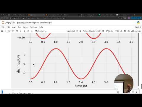
- Plots compare angular position θ, angular velocity θ̇, and angular acceleration θ̈; the linear and nonlinear curves develop different periods and drift out of phase.
- Angular velocity corresponds to tangential speed through v = Lθ̇, so a 1 m pendulum moving at 2 rad/s has a speed of 2 m/s.
- Students are asked to define an error measure and report where the difference appears, rather than relying only on visual inspection.
- At an initial angle of π radians, the nonlinear restoring term sinθ is zero, so an exactly upright rigid pendulum can remain at rest in the ideal model.
- That upright equilibrium is unstable: a small disturbance can make the pendulum fall and begin swinging.
- The linear approximation substitutes θ for sinθ, predicting a large acceleration near π; with L = 1 m, the magnitude is about πg, or 30 m/s².
- Cooper connects inverted-pendulum dynamics to Segways and hoverboards, where feedback-driven acceleration helps keep a rider upright.
- At 30° (π/6 radians), the linear and nonlinear curves still show a small period difference and a slight acceleration-amplitude difference.
- At 10°, the plotted curves nearly overlap, and the period difference is too small to distinguish with a stopwatch.
- The comparison illustrates that approximation error decreases as the initial angle approaches zero.
- Cooper suggests that 30° may be adequate for many estimates, while smaller angles make the linear model increasingly reliable.
- The period is one possible error metric: the 60° case shows a visible difference, while the 10° case is approximately 2 seconds for both models.
- Acceleration error can be estimated by comparing the linear term θ with the nonlinear term sinθ, scaled by g/L.
- A numerical difference can exist even when it is too small to measure experimentally, so the chosen error metric should match the task.
- Once θ and θ̇ are known, the radial force balance can be used to calculate string tension throughout the motion.
- Tension has two peaks per oscillation because the pendulum’s left-right motion is symmetric, giving matching behavior at positive and negative angles.
- Cooper closes by previewing angular momentum and its application to spinning-top design in the following week.
Transcript excerpt
0:00 streaming. Get this guy up there. Looks like we're live. Got microphone and probably need to relog into here. No, I'm good. So last time we were talking about like
0:55 what are the forces actually causing motion in a pendulum. Main things that we added on here were tension, gravity, and for the most part it's a pretty descriptive way of capturing like all the necessary like moving things. It doesn't have like amplitude reduction over time because there's no damping, there's no uh drag, there's no friction. It'll just keep oscillating forever. Um, but in this project, one of the main things that can change is are we considering the full equ like the full nonlinear equation of motion which Not a huge
1:45 difference, but are we considering nonlinear or linear equation? Um, so is is our pendulum a spring or is it a actual like swinging um sign function sort of thing. Am I logged in yet? Still connecting. What if I refresh it? Creating, registering, connecting. It's thinking about it. Okay.
2:41 And what we saw last time was that like the as the angle is getting bigger the time period like frequency is smaller, time period is longer. Um so when when does that become a thing? So, when can we say that this is true. Does
3:36 anyone know like do you have a rule of thumb for a small angle approximation? >> Yeah. >> [clears throat] >> or pi over 18. Really signs, cosiness, it's all it's all in radians. It's just if you put your calculator in degree mode, it takes the input, divides by 180, and multiplies by pi. Um, so there's an extra factor in there. So 10 degrees, what do we think? Small enough.
4:26 Small. Anything bigger than that is not small.
This is the start of the transcript. Save this video free for the whole transcript, searchable and time-coded.
In this course
Related notes
Summary, takeaways, and chapters were generated by AI from the video's transcript and may contain errors. The video belongs to its creator, Professor Ryan C. Cooper.