ME2120 - Dynamics

Overview

Ryan C. Cooper wraps up a spring-oscillation case study by connecting the system’s equations of motion to measured voltage signals. He explains phase plots, checks a predicted natural angular frequency of about 30 rad/s against a measured oscillation near 4.76 Hz, and shows how voltage amplitudes can be calibrated to displacement in millimeters.

Key takeaways

An undamped spring oscillator forms an ellipse in position-velocity phase space, while damping causes the trajectory to spiral toward equilibrium.
Measured voltage can be checked against a motion model without converting units by comparing oscillation periods; the case study’s predicted and observed periods are both about 0.21 seconds.
Angular frequency and ordinary frequency differ by a factor of 2π: 30 rad/s is about 4.8 Hz, which agrees closely with the measured 4.761 Hz.
A brief impulse sets the initial velocity through m v₀ = FΔt, and the resulting oscillation amplitude depends on impulse, mass, and natural frequency.
Voltage-to-displacement calibration can use known predicted amplitudes, such as approximately 76 voltage units corresponding to 5 mm in the x direction.

Chapters

0:00 Kinetics Recap: From Degrees of Freedom to Motion Equations

Cooper reviews the workflow: define degrees of freedom and position, then draw kinetic and free-body diagrams.
The diagrams lead to second-order equations of motion, which are solved using initial position and velocity.
For oscillatory solutions, imaginary roots in the characteristic equation produce sine and cosine terms.

3:00 Expressing Oscillator Position and Velocity as Functions of Time

Position is represented with time-dependent coordinate functions, such as x(t) and y(t), rather than as a single fixed value.
The position functions allow the system’s location to be evaluated at any chosen time.
Velocity is obtained by differentiating position with respect to time.

8:00 Differentiating Sinusoidal Position to Find Velocity

For a sinusoidal position function, differentiation produces a cosine velocity function.
The example velocity includes the oscillation amplitude multiplied by angular frequency, as in a term proportional to 5ω cos(ωt).
This derivative relationship explains why position and velocity reach their extrema at different times.

13:00 Spring-Oscillator Phase Plots: Ellipses Without Damping

At maximum positive or negative displacement, spring velocity is zero; at zero displacement, speed is greatest.
Undamped oscillation traces an elliptical path in position-velocity phase space, with direction indicating whether the mass moves left or right.
Damping makes the phase trajectory spiral toward the final equilibrium position as the system loses energy.

18:00 Connecting Predicted Motion to Measured Voltage Signals

After solving the differential equations, Cooper asks how the predicted time functions can be compared with measured voltage data.
Possible approaches include evaluating the functions at selected times, such as 0.25 or 0.5 seconds, or plotting prediction and measurement together.
The discussion identifies matching oscillation periods as a useful check even when voltage and displacement use different units.

23:00 Plotting the Predicted Oscillation and Checking Signal Amplitude

Cooper plots the model’s x(t) and y(t) functions and corrects the displacement scale to millimeters.
Signal comparison can test amplitude, frequency, and phase; plotting the curves together offers a visual check of overall agreement.
Extreme values of the measured signal can be compared with predicted displacement amplitudes.

31:00 Impulse, Initial Velocity, and Consistent Units

The y-direction coefficient comes from the initial velocity created by an impulse, using m v₀ = FΔt.
The resulting displacement coefficient depends on the impulse divided by mass and natural angular frequency, including a term proportional to FΔt/(mω).
Cooper cautions that a tiny 22 g object requires small impulse units: using a full newton-second impulse would imply an unrealistically large motion.

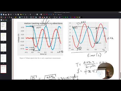
36:00 Estimating the Oscillation Period from Signal Graphs

The plotted signals complete about two cycles in 0.42 seconds, giving an estimated period of 0.21 seconds per cycle.
Counting zero crossings or comparing repeated peaks provides a practical way to estimate period from a noisy graph.
The measured voltage signal also has a period near 0.21 seconds, supporting the model’s predicted timing.

41:00 Converting 30 Rad/s to Hertz and Quantifying Frequency Error

Natural angular frequency is measured in radians per second, while ordinary frequency counts cycles per second in hertz.
Because one cycle is 2π radians, a predicted 30 rad/s corresponds to about 4.8 Hz, not 30 Hz.
The graph suggests roughly 5 Hz, close to the measured value of 4.761 Hz; Cooper discusses comparing the difference and reporting relative error.

48:00 Calibrating Voltage to Millimeters and Previewing the Pendulum Project

The x-direction calibration maps a voltage amplitude of about 76 to a predicted displacement amplitude of 5 mm.
The y-direction voltage amplitude of about 6 corresponds to the impulse-driven displacement amplitude FΔt/(mω); the two channel conversions may differ.
A point-by-point ratio of predicted values to measured voltages can estimate a steadier calibration factor despite measurement noise.
Cooper previews project three on a pendulum and case problem four on spinning-top design and 3D printing.

Transcript excerpt

0:47 Okay. All right. So, backing up again, wrapping up case study 3 today and we'll do quick tour of like where we're headed for rest of the semester because we're coming in to the end pretty fast. Sound good? uh recap of last class on Monday is we were working on kinetics. So kinetics is sort of like how is this thing moving or why is it moving and once we have definition once we know how many degrees of freedom there are we define what position is even if it's just saying like functions exist and then we have our kinetic diagram and free body diagram then we can actually set up our

1:35 equations of motion which are these second order differential equations And then we went through once you have those then you're actually like plugging in like okay here's my initial conditions let me find the natural frequency what's the initial position the initial velocity we went through did that we found x of t and y of t like here's our functions for yeah x of t and y of kind of nice looking good, right? And and this was just a a little side

2:26 note cuz someone was like, "How do you know it's signs and cosiness?" Um if you end up with imaginary numbers then in your in your characteristic equations then signs and cosiness. Cool. All right. So we've got let's just grab these two things. See if that works. So we set up the initial like hey this

3:30 is my definition for position because there are no vector differential equations like once there are like you can set them up as vectors but when it comes down to it functions are usually like um functions like this, right? Like some you plug in a t, you get an x or

This is the start of the transcript. Save this video free for the whole transcript, searchable and time-coded.

Related notes

Summary, takeaways, and chapters were generated by AI from the video's transcript and may contain errors. The video belongs to its creator, Professor Ryan C. Cooper.