ME2120-002
Overview
Professor Ryan C. Cooper develops the equations of motion for an Earth-orbiting point mass, using cylindrical coordinates and conservation of angular momentum to reduce two coupled nonlinear differential equations to a radial equation plus an algebraic relation for angular velocity. He derives the circular-orbit speed, about 3,074 m/s at a radius near 42 million meters, then uses Python's solve_ivp to verify constant radius and reconstruct the orbital path from the angle and radius.
Key takeaways
- For a point mass orbiting Earth, zero gravitational torque about Earth's center conserves angular momentum: mR² theta_dot stays constant.
- Angular momentum conservation lets the radial equation stand alone as a second-order differential equation, while theta_dot is recovered algebraically from radius.
- A circular orbit requires zero radial acceleration, giving v0 = sqrt(G M_E/R0); at a radius near 42 million meters, the speed is about 3,074 m/s.
- Numerical solvers such as solve_ivp handle a second-order equation by integrating two first-order equations for radius and radial velocity.
- Dimensional analysis can catch algebra errors: the angular-rate relation needs an R² denominator to produce units of radians per second.
- A planar orbital path can be reconstructed from polar data using x = R cos(theta) and y = R sin(theta), with sufficient time resolution and equal plot-axis scaling.
Chapters
- The class resumes Problem 3 after identifying degrees of freedom, kinematics, forces, and equations of motion.
- Cooper uses cylindrical coordinates, with radius R and angle theta, to describe a satellite moving relative to Earth.
- The system has two degrees of freedom and initially produces two coupled, nonlinear differential equations.
- The radial and theta equations each involve R and theta, so they are coupled rather than independent.
- Cooper considers summing moments about Earth and notes that gravity creates zero torque about Earth's center because its force points along the radius.
- A torque changes rotational motion, motivating an angular momentum equation as another way to simplify the system.
- For a point mass orbiting Earth, angular momentum is H = mR² theta_dot, using the satellite's mass rather than Earth's mass.
- With zero net moment about Earth, angular momentum remains constant: mR² theta_dot = mR0² theta_dot0.
- The conservation relation shows that increasing orbital radius decreases angular velocity, and decreasing radius increases it.
- Cooper substitutes theta_dot = R0² theta_dot0 / R² into the radial equation to eliminate the second differential equation.
- The resulting radial acceleration depends on R and the initial angular velocity, rather than requiring a separate second-order equation for theta.
- He corrects an accidental extra square in the derivation and emphasizes checking powers algebraically.
- The initial tangential speed is v0 = R0 theta_dot0, allowing the radial equation to be written without theta or theta_dot0.
- The radial equation becomes R_double_dot = -G M_E/R² + R0² v0²/R³, combining inward gravity with the outward radial effect of angular motion.
- Angular velocity remains recoverable from the algebraic conservation relation once the radius is known.
- For a circular orbit, constant radius requires radial velocity and radial acceleration to be zero.
- Setting R_double_dot to zero in the radial equation gives v0 = sqrt(G M_E/R0), the circular-orbit speed.
- Cooper uses an orbital radius of roughly 42 million meters, about 6 million meters of Earth radius plus 35 million meters of altitude.
- Using G approximately 6 × 10^-11 and Earth's mass approximately 6 × 10^24 kg, Cooper calculates a circular speed of about 3,074 m/s.
- The calculation is framed as a force-balance prediction that the satellite should maintain a circular orbit at the chosen radius.
- Python is introduced to numerically integrate the radial equation and test whether the radius actually stays constant.
- The second-order radial equation is converted into two first-order equations: dR/dt = v_R and dv_R/dt = the radial acceleration.
- SciPy's solve_ivp is used as an initial-value problem solver with starting radius R0 and zero initial radial velocity.
- The integration returns time samples and arrays for R and dR/dt; the radial acceleration code uses the R² gravity term and R³ angular term.
- The numerical solution shows R remains constant over integrations spanning 1,000 seconds and then 10,000 seconds.
- For a circular orbit, theta_dot is constant and can be recovered from angular momentum; Cooper catches a missing R² denominator by checking units.
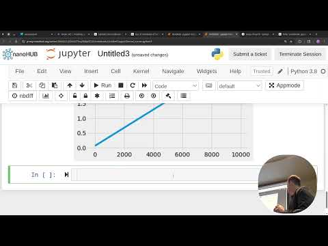
- The constant angular rate is approximately 10^-9 radians per second, and integrating it produces an angle that increases linearly with time.
- Cooper accumulates angle increments over evenly spaced time steps, then uses x = R cos(theta) and y = R sin(theta) to plot the orbit.
- The first plot looks distorted because the axes are not equal and the calculation uses too few time steps; increasing time resolution improves the path.
- The plotted trajectory resembles a circle, and the same numerical process can be repeated for other initial conditions and orbital paths.
Transcript excerpt
0:37 Okay. Welcome back. There we go. Do I have Does mic work? Mic works kind of. We can hear it. All right, how's that? Little louder. Nice. Cool. We are here in case problem number three. Last time Last time we did a lot of the engineering and kind of physics work. Identify Wait, the do degrees of freedom, kinematics,
1:27 kinetics, and then final step was actually getting to equations of motion. Everybody's ready, or do we need a minute to recollect? You want a minute? Everybody stand up. Stretch out. Get ready. Get pencils ready. don't want to do that. Ready to do some engineering? It's okay. It's good to check in with yourself and figure out what what am I ready for today? What are we ready for? Are we ready or not ready? It is April Fools. Yeah. There's nothing foolish about dynamics,
2:17 though. Oh, it is due next week. I did push it off, but it's not an April Fools' joke. Yeah, I did push it off, though. That one's not an April Fools' joke. I did push it off to Tuesday so we can have today and Friday to take a to like keep working on it. Yeah. Um Cool. Thanks for reminding me. Okay. So, we got to the point where we identified what forces are acting. We defined our acceleration. That was the step where through kind of like pulling teeth, I said like we're going to use cylindrical coordinates, and everyone's kind of like, "Uh,
3:04 I don't like those." But but we can use them. They work, and it's always the same definition. So, you the more you practice it, the more you're used to like defining terms in terms of like radius and angle starts to make sense. Uh or if you're a Laplace,
This is the start of the transcript. Save this video free for the whole transcript, searchable and time-coded.
In this course
Related notes
Summary, takeaways, and chapters were generated by AI from the video's transcript and may contain errors. The video belongs to its creator, Professor Ryan C. Cooper.