Lecture 20: advection diffusion equations, uPDE - part 1
Overview
The lecture develops the generic advection-diffusion-reaction equation, explains how constant-speed advection translates an initial condition and how nonlinear advection can form shocks, then demonstrates solving PDEs with the Python uPDE library. A hands-on 1D example shows that central differencing creates oscillations for advection, while upwind and flux-limiter schemes provide stable alternatives; the lecture ends by modeling shock formation with the inviscid Burgers equation.
Key takeaways
- Constant-speed advection has the exact solution f(x,t) = f₀(x − Ct), which translates the initial profile without changing its shape.
- For conservative advection written with flux F(f), the characteristic speed is F′(f); for the Burgers flux F(u) = u²/2, that speed is u.
- Central differencing is unsuitable for pure advection because its symmetric stencil mixes downstream information into the derivative and creates oscillations.
- First-order upwind is stable and monotone but introduces artificial diffusion; flux limiters such as van Leer and Superbee reduce smearing near steep gradients.
- uPDE lets users define a PDE, set initial and boundary conditions, and solve through a SciPy solve_ivp interface after spatial discretization.
- A spatially discretized PDE becomes a system of ODEs, enabling standard time integrators such as RK45 to advance the grid-point values.
Chapters
- Transport equations share unsteady, advection, diffusion, and source terms, even when the conserved quantity differs.
- The generic scalar transport equation can represent a passive tracer moving with a fluid, such as ink or particles.
- In chemical engineering, the source term often represents a reaction, yielding an advection-diffusion-reaction model.
- The total flux J includes both advective transport, commonly velocity times the transported quantity, and diffusive transport.
- A simple diffusion constitutive law uses a gradient, with the coefficient K potentially depending on time, space, or the field.
- K must remain inside the divergence operator when it varies, as thermal conductivity can vary with temperature.
- For one-dimensional advection, a constant speed C moves a signal without changing its shape when diffusion is absent.
- Positive C transports information left to right; negative C transports it right to left.
- A Gaussian pulse or step-shaped pollutant concentration should translate intact under pure constant-speed advection.
- When the advecting speed depends on the transported field, the equation becomes nonlinear and can develop shock-like behavior.
- For a flux form ∂t f + ∂x F(f) = 0, the characteristic speed is F′(f), not necessarily the flux factor itself.
- For Burgers’ equation with flux F(u) = u²/2, the true advecting speed is u.
- For constant C, the exact solution is f(x,t) = f₀(x − Ct), so each point retains the initial profile shifted by distance Ct.
- The transformation z = x − Ct moves the coordinate frame with the signal and reduces the PDE to no change in time.
- This derivation is an example of the method of characteristics, which converts PDE behavior into evolution along characteristic paths.
- Discretizing a PDE in space produces a collection of ODEs, one for each spatial grid point.
- SciPy’s solve_ivp can then integrate that system in time, while boundary conditions must be incorporated into the spatial discretization.
- The lecture introduces uPDE to handle these numerical details so users can focus on the governing physics.
- The uPDE workflow has three steps: define the PDE, constrain it with initial and boundary conditions, then solve.
- The library targets physics-focused users and supports single PDEs and coupled PDE systems in 1D and 2D, not 3D.
- Example applications include nonlinear diffusion, 2D mixing, diffusion-reaction systems, porous-media flow, combustion, and wave propagation.
- The classroom example imports the PDE class with `from upd import PDE`, alongside NumPy and Matplotlib.
- The lecture recommends upgrading the package to version 1.1 to access the newer advection `scheme` option.
- The example creates a 1D coordinate grid from 0 to π with 256 points and defines a field named `f`.
- The `add_advection` method takes an explicit velocity and a spatial scheme; in 2D, users specify x- and y-velocity components.
- The central scheme is selected initially to demonstrate its behavior, while upwind is the default.
- The library distinguishes this velocity-based term from a separate flux-form advection method.
- The `set_initial_condition` method accepts a constant, an array, or a callable function of space.
- The example compares a Gaussian pulse with a top-hat profile built from two Heaviside steps at x = 1 and x = 2.
- Periodic boundary conditions make the signal wrap around the domain, allowing repeated advection cycles.
- The PDE’s `solve` method wraps SciPy’s `solve_ivp` and accepts a time span, evaluation times, and integrator settings such as RK45.
- With speed 1 over a domain of length π, a run to 3.2 seconds captures approximately one trip around the periodic domain.
- The solution object exposes times and field arrays, which can be plotted at selected time indices to track the moving pulse.
- With central differencing, both the Gaussian and step initial conditions develop wiggles as they advect across the periodic boundary.
- The step profile becomes severely distorted even though its integral remains constant, showing that conservation alone does not guarantee an accurate shape.
- The observed oscillations are numerical artifacts, not physical behavior of the constant-speed advection equation.
- The central derivative uses values on both sides of a grid point, including downstream information that should not influence upstream advection.
- For advection-only problems, this centered stencil produces oscillatory, unstable solutions; RK45 can delay visible failure but does not fix the spatial scheme.
- A one-sided upwind stencil uses information from the direction the flow comes from.
- First-order upwind remains stable and avoids new oscillations, but its artificial diffusion gradually smooths sharp features.
- Flux-limiter schemes such as minmod, van Leer, Superbee, and MC reduce that smearing by using upwind behavior near steep gradients and higher-order behavior in smooth regions.
- For pure advection, the lecture recommends upwind or a limiter rather than central differencing; physical diffusion can also smooth numerical noise in advection-diffusion problems.
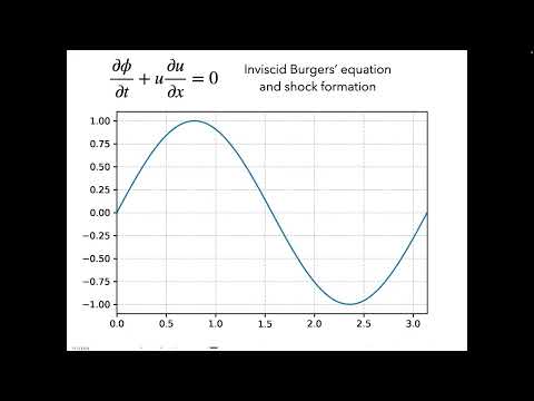
- The inviscid Burgers equation is nonlinear because the field u advects itself, and it serves as a simplified model for shock formation.
- In uPDE, setting the advection velocity to the field name `u` creates a field-dependent transport speed.
- A sine-wave initial condition on the 0-to-π domain steepens as positive and negative portions move toward one another, illustrating how a shock develops.
Transcript excerpt
0:00 Let's begin. There's two more slides left on on uh this lecture about conservation laws. Uh we're going to come back to these momentum equations, the Navis Stokes equations, I promise you. And we'll dig deeper into the details of the pressure, the gravitational term, the diffusion term. Um but all of these equations, they have a similar form. There's an unsteady term, there's an advection term, there's a diffusion term, and there's some source terms. Okay. Um, just remember what you're conserving. And for the Navis Stokes equations at least, there there's four equations and four unknowns like I said and remember in each term here, although you see a vector, but this is a divergence. So,
0:48 this turns into three terms. This turns into three terms and I show them in the next slide. Um and in the next slide this would be div uu div uvu vv and this is in a two-dimensional case actually. And so um I'll give you some homework to work these out. You seeing them will not register in your in your mind. You have to um work through them uh work through them by hand and try to get the details out of them. Um what will be more uh useful and what you will see most likely because probably not all of you are going to be doing um fluid mechanics etc. You'll just get the answer from a fluid solver but plug it in into your reaction system or into your viral
1:38 transport um whatever you're you're you're working through. Um so in that sense we will be working with the generic scale what we call the generic scalar transport equation. So going back if you take one step back and look at f as a conserved quantity or a derived
This is the start of the transcript. Save this video free for the whole transcript, searchable and time-coded.
In this course
Related notes
Summary, takeaways, and chapters were generated by AI from the video's transcript and may contain errors. The video belongs to its creator, Professor Saad Explains.