lecture 14: ODEs - Part 4

Overview

The lecture explains how time-scale separation makes ODE systems stiff, why SciPy’s explicit solvers suit non-stiff problems while implicit methods such as BDF and Radau handle stiffness more efficiently, and how to choose among solve_ivp methods. It then derives and simulates the SIR epidemic model using compartment balances and parameters β and γ, before introducing boundary-value problems and finite-difference approximations for spatial derivatives.

Key takeaways

A stiff ODE combines widely separated time scales; explicit solvers may then be forced into many tiny stability-limited steps, while implicit methods such as BDF or Radau can advance more efficiently.
In SciPy solve_ivp, RK45, RK23, and DOP853 are explicit choices, while BDF and Radau are implicit; LSODA can detect stiffness and adapt its method.
The basic SIR model follows conservation S + I + R = N and uses dS/dt = −βSI/N, dI/dt = βSI/N − γI, and dR/dt = γI.
In the SIR interpretation, β controls the rate of new infections and can represent interventions such as social distancing; γ = 1/D corresponds to an average infectious period of D days.
For a uniform spatial grid, the central first-derivative stencil is second order, so halving Δx reduces its error by roughly fourfold, compared with a twofold reduction for a first-order forward or backward stencil.
Finite-difference approximations turn boundary-value differential equations into coupled algebraic systems by relating unknown values at neighboring grid points.

Chapters

0:00 Stiffness as Separation Between Slow and Fast Time Scales

Stiffness reflects a large ratio of slow to fast time scales; the ratio is dimensionless, and values around 1,000 or greater are a practical warning sign.
A system is not stiff merely because it is fast or slow: reactions all occurring on microsecond scales can be non-stiff if their time scales are comparable.
The Van der Pol oscillator illustrates stiffness through gradual motion interrupted by sharp changes; sound traveling near 300 m/s alongside air motion near 1 m/s is another example of separated scales.

4:14 Why Explicit and Implicit ODE Solvers Behave Differently

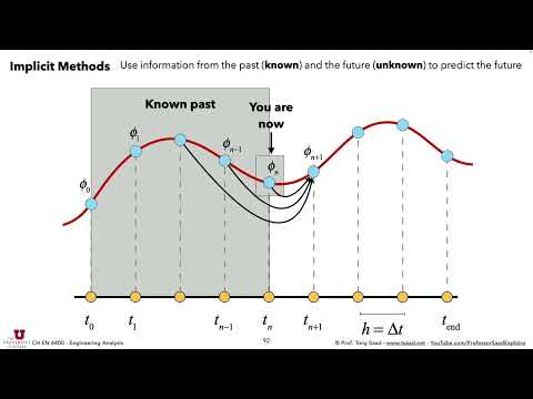
Explicit methods advance using previously computed values, making them efficient for non-stiff systems but conditionally stable and potentially inefficient for stiff systems.
Implicit methods include the unknown future value, creating an equation that generally requires a nonlinear solve but can remain stable with larger time steps.
For stiff problems, explicit methods may take enormous numbers of tiny steps to preserve stability, even while the solution changes slowly.

9:56 Choosing SciPy solve_ivp Methods for Stiffness

SciPy’s default RK45, RK23, and DOP853 are explicit Runge–Kutta methods; DOP853 is an eighth-order option for high-precision non-stiff calculations.
Radau and BDF are implicit choices for stiff systems; BDF is a backward differentiation formula method with orders one through five.
LSODA automatically detects stiffness and switches between suitable approaches; unusually many iterations or solver failure with RK45 can indicate that BDF or Radau is worth trying.
Higher-order methods can reduce error faster as step size shrinks, but typically cost more per step.

14:20 SIR Epidemics as a Compartment-Model Example

The SIR model tracks a fixed population divided into susceptible (S), infected (I), and recovered (R) groups, with S + I + R = N.
People move from susceptible to infected and then from infected to recovered; the resulting curves show infection growth, a peak, and eventual decline as susceptible people are depleted.
The model provides a foundation for adding features such as hospitalization, vaccination, and social-distancing policies.

20:25 Compartment Models Use Inflow Minus Outflow

For any compartment, its rate of change is the rate entering minus the rate leaving, as illustrated by tracking shoppers entering and exiting a department store.
The store’s population balance can include an outflow proportional to the number inside and an inflow related to the population outside.
Building a compartment model means defining the groups, identifying each transition, and connecting the inflows and outflows.

25:15 Deriving the SIR Infection Rate and βSI/N

The susceptible group loses people only through infection in the basic SIR model, so dS/dt is the negative of the infection transition rate.
With I infected people in a total population N, the fraction I/N represents the chance of encountering an infected person; multiplying by S gives the susceptible-infection interaction term.
The transmission parameter β scales that interaction, producing an infection flow of βSI/N and dS/dt = −βSI/N.

31:00 Modeling Recovery with γ and Completing the SIR Equations

Infected people enter through the infection flow βSI/N and leave through recovery, modeled as γI.
The recovery parameter γ has units of inverse time: if the infectious period is D days, a simple estimate is γ = 1/D per day.
The complete system is dI/dt = βSI/N − γI and dR/dt = γI, with recovered people receiving the infected group’s outflow.

34:27 Implementing the SIR System with SciPy solve_ivp

The worked setup uses a population N = 1,000, initial infection I₀ = 10, R₀ = 0, β = 0.5, and γ = 1/14 per day.
The initial susceptible count is set by conservation, S₀ = N − I₀ − R₀; the state vector and returned derivatives must use the same S, I, R order.
A Python right-hand-side function returns the three SIR rates, and solve_ivp integrates them over 100 days with requested output times for plotting.
The example uses the standard explicit solver because this parameter set does not require an implicit stiff solver.

45:45 How β Changes the Timing and Height of an Epidemic Peak

Increasing β raises the infection flow βSI/N, moving the infected curve’s peak earlier and typically making it taller.
With β = 0.8, the demonstration peaks in roughly 10 days at about 700 infected people; reducing β to 0.1 produces a lower, slower curve that requires a longer simulation.
Social distancing can be represented as a reduction in effective β, flattening the infection curve without directly creating immunity.

50:18 How Recovery Rate γ Affects Infections and Curve Shape

A larger γ shortens the infectious period, moving recovery earlier and reducing the time infected people can transmit disease.
Changing recovery from 14 days to 5 days (γ = 1/5 per day) lowers the demonstrated infected peak from about 400 to about 200.
A 28-day infectious period keeps people infectious longer; under the model’s assumption that they continue mixing, infections become more concentrated into a high peak rather than necessarily extending the epidemic.

55:45 Boundary-Value Problems Require Conditions at Spatial Boundaries

Initial-value problems start from a known state and integrate forward in time, whereas boundary-value problems prescribe conditions at spatial boundaries.
A one-dimensional rod with temperatures fixed at both ends is a boundary-value problem; the interior temperature profile must satisfy the governing physics and those endpoint conditions.
SciPy’s solve_bvp is presented as limited and inconvenient for general use, particularly beyond one spatial dimension, motivating a finite-difference approach.

1:01:00 Discretizing a Spatial Domain for Finite Differences

Finite differences divide a spatial domain into grid points separated by h or Δx and approximate derivatives using neighboring unknown values.
Writing f(xᵢ) as fᵢ converts derivative expressions into algebraic relations among grid values.
Because neighboring grid values are coupled by derivative approximations, the discretized boundary-value problem becomes a system of algebraic equations that can be solved.

1:04:50 Forward, Backward, and Central First-Derivative Formulas

The forward difference, (fᵢ₊₁ − fᵢ)/Δx, and backward difference, (fᵢ − fᵢ₋₁)/Δx, are first-order approximations and can use locally varying spacing.
The central difference, (fᵢ₊₁ − fᵢ₋₁)/(2Δx), is second order and requires uniform spacing across the points in the formula.
Halving Δx typically halves first-order error but reduces second-order central-difference error by about a factor of four.
Higher-order biased formulas are useful in directional-flow problems where the approximation should draw information from the upstream side.

1:08:58 Second-Derivative Stencils and Course Project Guidance

The standard central approximation for a second derivative is (fᵢ₊₁ − 2fᵢ + fᵢ₋₁)/Δx², a second-order stencil used in the earlier heat-transfer problem.
Forward- and backward-biased second-derivative formulas can use additional grid points, with higher-order stencils trading wider neighborhoods for improved accuracy.
The next topic is truncation-error order; students are also directed to prepare five-minute project presentations followed by two minutes of questions and to contact the instructor through Canvas.

Summary, takeaways, and chapters were generated by AI from the video's transcript and may contain errors. The video belongs to its creator, Professor Saad Explains.