Lecture 15: ODEs part 5 - Boundary Value Problems BVPs
Overview
Boundary value problems (BVPs) are solved by discretizing spatial derivatives with finite differences, turning a continuous ODE into a system of algebraic equations. The lecture derives second-order central-difference equations for Dirichlet and Neumann conditions, eliminates Neumann ghost points, and demonstrates a NumPy solution with `np.linalg.solve`, then extends the procedure to advection-diffusion and nonlinear radiation problems.
Key takeaways
- A finite difference BVP is built by applying the continuous governing equation at discrete spatial points and replacing derivatives with algebraic approximations.
- For a second-order finite difference method, halving the grid spacing ideally reduces truncation error by a factor of four.
- Neumann conditions introduce an out-of-grid ghost value when central differences are used at a boundary; discretizing the boundary derivative lets that value be eliminated.
- Dirichlet conditions specify a variable's boundary value, while Neumann conditions specify its slope or flux, and each changes the boundary equation in a different way.
- In a mixed-order discretization, the least accurate derivative approximation generally sets the order of the overall numerical error.
- Nonlinear BVPs, such as radiation heat-transfer models, require residual equations and a nonlinear root solver instead of a linear solve.
Chapters
- Initial value problems typically specify conditions in time, while boundary value problems specify values or fluxes at spatial endpoints.
- A heat-conducting rod is a one-dimensional BVP: endpoint temperatures are known, and the temperature profile between them is unknown.
- Finite difference methods extend the course's earlier matrix-based approach to boundary problems and can support multidimensional problems beyond one-dimensional solvers.
- Divide the spatial interval into discrete points with spacing Δx, then solve for the dependent variable, such as temperature, at each point.
- Numerical calculus provides several choices, including central, forward, and backward differences for first and second derivatives.
- The standard second derivative approximation uses neighboring values: (fᵢ₋₁ − 2fᵢ + fᵢ₊₁)/Δx².
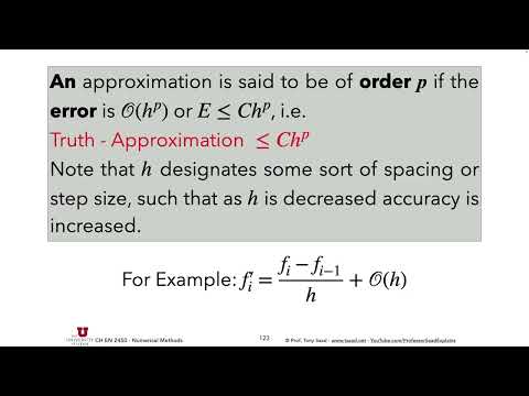
- A method has order P when its truncation error scales as O(Hᴾ), where H is the grid spacing or another refinement measure.
- Halving H halves the error for a first-order method, but reduces it by a factor of four for a second-order method.
- The order describes approximation error, not derivative order: a first-derivative approximation can have second-order accuracy.
- When discretizations of different orders are combined, the lowest-order term generally controls the overall error.
- For the heat-transfer model T″ = h(T − T∞), the continuous equation applies at every point, including the selected grid points.
- Substituting the second-order central difference gives a discrete equation involving Tᵢ₋₁, Tᵢ, and Tᵢ₊₁.
- Applying that equation at the interior points and inserting known endpoint temperatures produces a linear system with one equation per unknown.
- The resulting coefficient matrix is tridiagonal, with lower, main, and upper diagonals assembled and solved using linear algebra.
- A Dirichlet boundary condition fixes the dependent variable, such as a specified temperature at a rod endpoint.
- A Neumann boundary condition fixes a derivative or flux, such as the rate of heat entering or leaving a boundary.
- Flux conditions can be more practical than fixed values in applications such as heat transfer and flow, where controlling a rate may be easier.
- Applying the central-difference governing equation at the right boundary introduces a fictitious value Tₙ₊₁ outside the grid.
- Discretize the Neumann condition as (Tₙ₊₁ − Tₙ₋₁)/(2Δx) = β, then use it to eliminate Tₙ₊₁.
- The boundary equation then relates only grid unknowns, closing the system without adding a real degree of freedom.
- The resulting matrix changes at the boundary, including a final lower-diagonal coefficient of 2 and an adjusted right-hand side.
- The coding task is compact, but engineers still need to understand how the governing equation and boundary condition produce each matrix entry.
- A numerical result from a tool or AI is difficult to assess without understanding concepts such as linear systems and Neumann conditions.
- The procedure generalizes: discretize the governing equation, discretize any Neumann condition, and combine them to remove out-of-domain values.
- The Jupyter example uses 100 points on x ∈ [0, 1], an effective heat-transfer coefficient of 1, Tleft = 100 K, and T∞ = 500 K.
- NumPy builds the tridiagonal matrix and right-hand side, while `np.linalg.solve` computes the temperature profile and Matplotlib plots it.
- Changing the prescribed slope β checks the boundary behavior: positive β raises the profile near the right edge, negative β lowers it, and β = 0 gives an approximately flat, insulated boundary.
- The first matrix row enforces Tleft directly; the final row encodes the Neumann condition through the ghost-point elimination.
- For U″ = x²U, the left boundary specifies U′(0) = α and the right boundary fixes U to β.
- A central derivative approximation gives (U₂ − U₀)/(2Δx) = α, so the ghost value becomes U₀ = U₂ − 2αΔx.
- Substituting that expression into the discretized equation removes U₀ and yields a closed system with the right Dirichlet condition.
- The steady advection-diffusion example combines a second derivative for diffusion with a first derivative for advection.
- Both derivative terms can be approximated using formulas from the numerical-calculus table, then assembled into an algebraic system.
- Using a first-order approximation for one term and a second-order approximation for another makes the overall error first order, because the lower-order term dominates.
- Radiation makes the heat-transfer equations nonlinear in temperature, so discretization produces a nonlinear system rather than a linear matrix equation.
- Form one residual per grid point, including boundary residuals such as T₁ − Tleft, and solve the residual system with a root-finding method.
- A Neumann boundary can also be incorporated by eliminating the ghost point and using the resulting boundary equation as the final residual.
Transcript excerpt
0:00 Let's begin. This is the last part of our ordinary differential equations discussion before we embark on part three with conservation laws and partial differential equations. If you remember with ODEs, we classify them as initial value problems. You need an initial condition and boundary value problems where the boundary of the system in question is specified and you need to understand what's happening spatially between those boundaries. Um with ODEs, we're limited to one dimension by definition because there's only one independent variable. For initial value, it's usually time. For boundary values, it's usually space. We call it X or could be any other um independent variable. It's just one independent variable.
0:48 And the classic example we did was the heat transfer in a rod. So, we did this early on at the beginning with systems of linear equations. This was a great example um for how we obtain these systems of linear examples. In this case, there is um temperatures specified at the ends of this material. Heat is only um being transferred along the rod, not vertically because you can assume it's a very thin rod or changes in the vertical direction are insignificant. You can assume it's just unidirectional in the in this X direction and there's some sources. There's radiation. We We did this with um with a heat source. We did this with advection. We did this with radiation.
1:37 Um so, different things on the right-hand side, but the point is this is a one-dimensional problem in space with two uh fixed boundary points, okay? Or more. You could have more depending on the order of the differential equation. Um uh but in this case, uh this is a second-order ODE and we talked about the classification of these ODEs. Whether in time or space, they have the same
This is the start of the transcript. Save this video free for the whole transcript, searchable and time-coded.
In this course
Related notes
Summary, takeaways, and chapters were generated by AI from the video's transcript and may contain errors. The video belongs to its creator, Professor Saad Explains.