Lecture 16: vector calculus - Part 1
 Watch on YouTube →
Overview
Professor Saad connects vector calculus to the course’s upcoming conservation laws and partial differential equations, reviewing scalar and vector fields, vector operations, and the gradient’s meaning. The lecture also demonstrates Python tools including NumPy meshgrid, gradient, and Matplotlib contourf and quiver, emphasizing array indexing and coordinate-spacing details needed to compute and visualize fields correctly.
Key takeaways
- Conservation equations for mass, momentum, and energy rely on vector calculus, making its differential and integral operators foundational for deriving engineering PDEs.
- NumPy meshgrid turns 1D coordinate arrays into 2D coordinate matrices; with the standard layout, Cartesian index [i, j] corresponds to matrix index [j, i].
- A contour line marks a constant scalar-field value, while contour colors encode field magnitude and make 2D peaks and troughs easier to read than a 3D surface plot.
- The gradient of a scalar field is a vector pointing toward the steepest local increase; a zero gradient at a flat point does not by itself establish whether that point is a minimum, maximum, or saddle.
- For standard meshgrid arrays, passing coordinates to np.gradient in y, x order yields derivatives in y, x order; reorder them to x, y before using them as Cartesian quiver components.
- A vector-field component is a scalar field over the full domain: for example, the x-component of velocity can depend on x, y, z, and time.
Chapters
- The course turns from regression, interpolation, and nonlinear equations toward conservation laws and partial differential equations.
- Vector calculus provides tools needed to derive mass, momentum, and energy equations, including the Navier-Stokes equations.
- The lecture reviews scalar and vector fields, gradient, divergence, curl, and integral theorems.
- A scalar field assigns one direction-independent value to every continuum point; density, temperature, and pressure are examples.
- Time-dependent fields are commonly shown as animations rather than as an additional plotted axis.
- A contour plot encodes a two-dimensional scalar field’s value as color, making peaks and troughs easier to interpret than a 3D surface.
- A one-dimensional x array and a one-dimensional y array do not directly provide coordinate pairs for evaluating a 2D field.
- NumPy’s meshgrid combines the coordinate arrays so each grid location has corresponding x and y values.
- The lecture uses the two-variable function cos(3x) + sin(4y) to motivate evaluating fields over a full plane.
- np.meshgrid accepts 1D coordinate arrays and returns 2D coordinate arrays, conventionally named xx and yy.
- The x coordinates repeat across rows while the y coordinates repeat across columns in the standard meshgrid layout.
- For a Cartesian point at indices i and j, the corresponding matrix entry is accessed as [j, i], reflecting row-column indexing.
- The live Python example creates x and y with np.linspace, then calls np.meshgrid(x, y) to generate coordinate matrices.
- Matplotlib’s imshow can display an array as colored pixels; origin='lower' puts the origin at the conventional lower-left.
- The colorbar maps displayed colors back to array values, illustrating how repeated rows or columns represent constant coordinates.
- The Taylor-vortex example evaluates a function on 2D xx and yy arrays; passing incompatible 1D arrays of 100 and 200 points causes a shape mismatch.
- plt.contourf(xx, yy, z) plots filled contours, while increasing the levels argument adds more contour intervals.
- Each contour line represents locations where the scalar field has a constant value; aspect ratio affects how the plot’s geometry appears.
- A scalar field can be written as a function of position and time, such as temperature T(x, y, t) in a 2D unsteady diffusion problem.
- A vector combines related directional components, such as x-, y-, and z-momentum, rather than arbitrary values like density, temperature, and pressure.
- Vector components can each depend on every spatial coordinate and time, even when a component points along only one coordinate direction.
- Vector addition and subtraction operate component by component, producing another vector.
- The dot product sums componentwise products and returns a scalar; it is zero for perpendicular vectors and can be negative for opposing directions.
- The cross product returns a perpendicular vector in 3D, follows the right-hand rule, vanishes for parallel inputs, and reverses sign when its operands are swapped.
- Cartesian unit vectors i, j, and k form a basis, with self dot products of 1 and pairwise dot products of 0.
- A vector field assigns a vector to each position and time, and each component of that vector is itself a scalar field.
- Velocity components u, v, and w can vary with x, y, z, and t rather than depending only on their corresponding coordinate.
- Vector-field visualization is harder than scalar-field plotting because each plotted location also needs an arrow direction and magnitude.
- The nabla, or del, operator is written as a vector of partial derivatives: ∂/∂x, ∂/∂y, and ∂/∂z.
- Nabla is an operator, not a completed result: it must act on a scalar, vector, or other quantity to produce an output.
- For a constant α, nabla(αf) equals α nabla(f), and nabla distributes over sums; a variable factor cannot generally be taken outside the derivatives.
- The gradient of a scalar field f is ∇f = (∂f/∂x, ∂f/∂y, ∂f/∂z), so its result is a vector.
- At a point, the gradient points in the direction of the greatest local increase in f; the negative gradient points toward greatest decrease.
- Gradient direction is local information and does not guarantee that a search has found a global maximum or minimum.
- In one dimension, the gradient reduces to df/dx, with a positive derivative pointing toward increasing x and a negative derivative pointing backward.
- At a locally flat point, df/dx is zero, so the gradient alone does not indicate which way to move next.
- Gradient-based optimization methods use derivative direction to seek minima or maxima, but may need additional checks near flat regions.
- The example builds a 5-by-5 spatial domain with 64 points in each direction and creates its coordinate arrays using np.linspace and np.meshgrid.
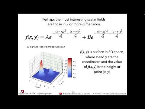
- Two Gaussian peaks are placed at roughly one-third and two-thirds of the domain, each with standard deviations of 0.5.
- The second peak is assigned half the amplitude of the first, and imshow or contourf displays the resulting scalar field.
- np.gradient computes array derivatives using second-order accurate central differences in the interior.
- Coordinate spacing must be supplied when grid intervals differ from 1; the lecture passes the 1D coordinate arrays rather than only the field array.
- With standard meshgrid matrix layout, the call uses y before x, and the returned derivatives are ordered ∂f/∂y then ∂f/∂x.
- Those derivative outputs must be reordered when assigning Cartesian gradient components to a vector plot.
- plt.quiver plots arrows at x-y locations, using the gradient’s x and y components to define each arrow’s direction.
- A dense 64-by-64 arrow field can obscure the scalar contours, so reducing resolution or skipping arrows makes the direction pattern clearer.
- Around each Gaussian peak, arrows point toward increasing field values; homework will combine spatial discretization with solving an initial-value problem.
Transcript excerpt
0:00 Let's begin. We're going to hit our last portion of the course and I call that conservation laws and partial differential equations. And this will set the so far what we've done. We've learned mostly tools and tricks that could get you to do your research. Most of your research doing data analysis. you're going to be using regression, interpolation, um non you're solving a nonlinear equation, you have all of those tools under your belt, at least a a an exposure to those tools that can get you started. So that's that's the primary the one of the objectives of the course. The second objective is to get you prepped into some core chemical engineering concepts. Not all of you
0:48 remember those or might have seen those because you might be coming from a different discipline. So this is the opportunity um to enforce those concepts and introduce those concepts to you. But I do expect you to have taken the bridging course in the summer if you're coming from a different discipline. So this will reinforce those concepts again. Um now with partial differential equations uh partial differential equations will represent conservation laws and and to do partial differential equations we cannot do them without vector analysis and vector calculus. Um and if you remember I told you that partial differential equations are the tuning forks of engineering science. Vector calculus is the tuning fork of partial
1:35 differential equation. I love the tuning. I love that analogy. Okay. So, it's it's it's essential to review vector calculus. Who's I expect that all of you have done some vector calculus in the past. Can can I see some hands? Okay, great. So, you you know what a vector is, etc. This is this is what I'm going to begin with. I'm going to assume
This is the start of the transcript. Save this video free for the whole transcript, searchable and time-coded.
Related notes
Summary, takeaways, and chapters were generated by AI from the video's transcript and may contain errors. The video belongs to its creator, Professor Saad Explains.