Lecture 17: Vector Caculus - Part 2
Overview
The lecture develops practical visualization techniques for scalar gradients, then connects vector-calculus operators to measurable physical behavior. It defines directional derivatives, divergence, the Laplacian, and curl, using a moving temperature-sensing drone, fluid flow through a small box, and neighboring function values to explain their roles in transport and flow analysis.
Key takeaways
- A directional derivative is the gradient projected onto a unit direction, so it measures scalar change per unit distance without depending on the arbitrary length of the direction vector.
- For a sensor moving through a steady spatial field, the measured time rate is velocity dotted with the field's gradient; the chain rule adds a direct partial-time term when the field itself changes over time.
- Divergence is local net volumetric outflow per unit volume: positive means net outflow, negative means net inflow, and zero means balanced inflow and outflow.
- Incompressible fluid flow satisfies ∇·u = 0, but this condition does not mean the velocity field itself is zero.
- The Laplacian compares a field's value with neighboring values: zero corresponds to local averaging, positive curvature can indicate a minimum, and negative curvature can indicate a maximum.
- Curl measures local rotation; for a two-dimensional velocity field its rotational component points in the z direction, and zero curl identifies an irrotational field.
Chapters
- Set Jupyter's inline figure format to SVG so plots remain sharp when zoomed, unlike raster PNG or JPEG images.
- Export publication figures as SVG or PDF when possible; converting a raster image to PDF does not make it vector-based.
- The SVG setting applies to plots throughout a Jupyter notebook and improves figure clarity in papers.
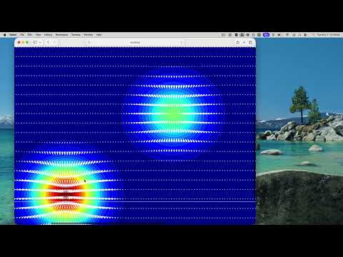
- Use Python slice objects to subsample the X and Y grids and the gradient components before passing them to Matplotlib's quiver plot.
- Adjust the slice step, such as skipping every third or fifth grid point, to reduce crowded arrows.
- Change the contour plot's colormap, for example to jet or magma, and increase the contour levels to create smoother color bands.
- Increase quiver's scale value to shrink arrows and make their relative direction and size easier to inspect.
- For a scalar field, the gradient components give slopes along the coordinate axes, such as x and y in Cartesian coordinates.
- The full gradient points in the direction of steepest increase, but its individual components do not directly give the slope along an arbitrary path.
- A hiker on a topographic map or a sensor moving off-axis needs the rate of change in a chosen direction.
- For a direction vector s, compute the directional derivative as the unit vector s/|s| dotted with the gradient of the scalar field.
- Normalizing s ensures the result describes slope per unit distance rather than scaling the slope with the length of the chosen vector.
- For a temperature field, the result is a scalar field whose values give the slope at each location along directions such as 2i + 3j.
- The directional derivative has units of the scalar field divided by length, matching the units of a spatial slope.
- A drone moving through a steady lake temperature field measures temperature as a function of time, even though the field varies only with position.
- For drone velocity u, the rate measured along its trajectory is u dotted with the temperature gradient; velocity is not normalized because speed affects the rate.
- The chain rule gives df/dt = (∂f/∂x)(dx/dt) + (∂f/∂y)(dy/dt), equivalent to velocity dotted with the gradient.
- If the field also changes directly with time, add the partial time derivative; this sets up the material derivative used in transport equations.
- Define divergence as ∇·u, the dot product of the nabla operator with a vector field.
- In Cartesian coordinates for u = (u, v, w), divergence is ∂u/∂x + ∂v/∂y + ∂w/∂z.
- Because divergence is a dot product of two vectors, its result is a scalar with no direction.
- The same operator applies to velocity, electric, and magnetic fields, though fluid flow provides an intuitive physical example.
- Consider a tiny rectangular fluid volume with dimensions Δx and Δy and unit depth, aligned with the Cartesian axes.
- Only velocity components normal to each face contribute to flow across that face; tangential components do not cross the boundary.
- Let the x-face velocities differ by Δu and the y-face velocities differ by Δv, representing local changes across the box.
- Comparing inflow and outflow across all four faces isolates the net volume flow through the small region.
- The box's net outflow is ΔuΔy + ΔvΔx for unit depth, obtained by subtracting inflow from outflow on opposing faces.
- Divide net outflow by box volume ΔxΔy, then let the dimensions approach zero to obtain ∂u/∂x + ∂v/∂y.
- Thus, divergence measures local net volumetric outflow per unit volume, not the total flow rate through a finite surface.
- A positive value indicates net outflow, a negative value indicates net inflow, and zero means inflow balances outflow.
- For an incompressible fluid, ∇·u = 0: fluid entering a local region must leave it rather than accumulate through compression.
- Zero divergence does not mean zero velocity; it means the local net outflow is zero.
- For non-fluid fields, zero divergence is also called divergence-free or solenoidal.
- Divergence connects to flux through the divergence theorem, which equates integrated divergence over a volume with flux across its boundary.
- Apply divergence to the gradient of a scalar field to obtain the Laplacian, written ∇²f or Δf.
- In Cartesian coordinates, the Laplacian sums the scalar's second derivatives, such as ∂²f/∂x² + ∂²f/∂y² + ∂²f/∂z².
- The Laplacian maps a scalar field to another scalar field and appears in heat-transfer and other spatial transport equations.
- The lecture relates the sign of the Laplacian to local curvature: positive values rule out a local maximum, while negative values rule out a local minimum.
- In one dimension, the second derivative is approximated by [f(a+h) - 2f(a) + f(a-h)]/h².
- If the second derivative is zero, the value at a is the average of its two neighboring values; this is the local averaging intuition behind the Laplacian.
- If f(a) is below the neighboring average, the second derivative is positive and a local minimum is possible; if it is above, a local maximum is possible.
- A function whose Laplacian is zero everywhere is called harmonic.
- Curl is the cross product of the nabla operator with a vector field, and its result is another vector.
- For fluid velocity, curl is related to rotation and is the vorticity vector; in two dimensions, the nonzero component points along the z-axis.
- In 2D, the z-component is ∂v/∂x - ∂u/∂y; its sign indicates the rotational direction under the usual coordinate convention.
- A field with curl equal to zero is called irrotational, a condition that can simplify fluid-mechanics analysis.
- The lecture closes by previewing volume and surface integrals that connect the local operators to whole regions and their boundaries.
- The divergence theorem will formalize the relationship between divergence integrated over a volume and flux across its surface.
- Gradient, divergence, the Laplacian, and curl are introduced as tools that will support later transport-equation derivations.
Transcript excerpt
0:00 What I want to do now is I want to pick up where we left off with the gradient visualization uh and show you last time when we did the gradient visualization it looked pretty ugly. Um I want to show you a couple of tricks now so we can make it look a little beautiful. Unfortunately I already implemented the changes. So I'm going to try to trace uh to trace back what I did. Um, if you want to open up your notebook from last time and come on, if you open up your notebook from last time, uh, we clean this up first. So, I'll revert back to where we were last time. So,
0:47 first I want you to add these two lines. It took me a while. I should have shown you these early in the semester. Uh just type these in and put them in in all your Jupyter notebooks. So add these two lines to your boiler plates. Particularly this one percent config inline backend trigger format is SVG. What this is telling Jupiter um if you've taken my earlier my previous courses you know why I do this. If not please do yourself a service and add this line all the time. What this does, it makes all your figures in your Jupyter notebook turn into what's called scalable vector graphics. Okay, so by default images show up as what we call raers, pixelated pictures. Okay, but
1:37 open a word document for example and zoom in as much as you can. You can still see the font nice and crisp. Why? Because the computer is redrawing that font at very high resolution every time. That's called a scalable vector graphic format. Okay, it's still a graphic. You can do this with figures as well. Okay,
This is the start of the transcript. Save this video free for the whole transcript, searchable and time-coded.
In this course
Related notes
Summary, takeaways, and chapters were generated by AI from the video's transcript and may contain errors. The video belongs to its creator, Professor Saad Explains.