Fri Nov 20 2026 Lecture (L33) Stewart Section 5.3 The Evaluation Theorem
Overview
Mark Barsamian introduces the Evaluation Theorem in Stewart Section 5.3: for continuous f with antiderivative F, the definite integral from a to b equals F(b) minus F(a). He uses it to replace limits of Riemann sums with antiderivative calculations, confirming the area under 1/x from 1 to 7 is ln(7), approximately 1.946, and demonstrating the Net Change Theorem with a motion problem.
Key takeaways
- For continuous f with antiderivative F, the Evaluation Theorem computes the definite integral on [a, b] as F(b) − F(a).
- The signed area under 1/x from 1 to 7 is exactly ln(7), approximately 1.946, validating a Riemann-sum estimate near 1.95.
- An integral measures signed area: portions below the x-axis subtract from portions above it, as shown by the value 3 for x/2 − 2 on [2, 8].
- The Net Change Theorem says integrating a rate F′ over an interval gives the change F(b) − F(a) in the accumulated quantity.
- For velocity t² − 2t − 8 from t = 3 to t = 6, displacement is 12 feet even though the motion changes direction during the interval.
Chapters
- Mark Barsamian reviews Section 5.1's use of left and right rectangles to estimate signed area.
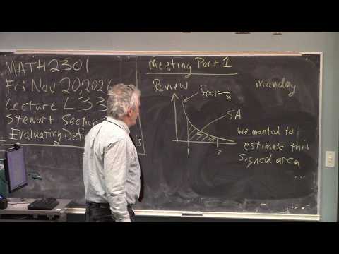
- The recurring example is f(x) = 1/x on the interval from x = 1 to x = 7.
- With more rectangles, the estimated area approaches approximately 1.95.
- Sigma notation represents adding the areas of n equal-width rectangles, each with width Δx and a function-value height.
- For a left sum, rectangle heights use x-values from x₀ through xₙ₋₁; the right sum uses x₁ through xₙ.
- Left and right sums both approach about 1.95 for 1/x from 1 to 7 as n increases.
- The definite integral from a to b is defined through the limit of Riemann sums as n approaches infinity, when the limit exists.
- Left, right, midpoint, and trapezoidal sums are different approximations that can converge to the same integral.
- Geometrical examples from the prior class illustrate evaluating signed area without explicitly calculating a sum limit.
- For continuous f on a closed interval [a, b], if F is an antiderivative of f, then the integral of f from a to b equals F(b) − F(a).
- The theorem turns a definite integral, defined by a limit of sums, into an endpoint calculation using an antiderivative.
- Barsamian contrasts this practical method with deriving integrals directly from Riemann-sum limits, a more advanced calculus technique.
- For f(x) = 1/x, an antiderivative on the interval [1, 7] is ln|x|.
- Evaluating endpoints gives ln|7| − ln|1| = ln(7), since ln(1) = 0.
- The exact value ln(7) is approximately 1.946, matching the earlier Riemann-sum estimate of about 1.95.
- For f(x) = x/2 − 2 on [2, 8], an antiderivative is F(x) = x²/4 − 2x.
- The endpoint calculation F(8) − F(2) gives 0 − (−3) = 3.
- The result matches the geometric signed-area calculation, where regions above and below the x-axis contribute with opposite signs.
- Rewriting the Evaluation Theorem as the integral of F′ from a to b equals F(b) − F(a) gives the Net Change Theorem.
- For velocity v(t) = t² − 2t − 8, displacement from t = 3 to t = 6 is the integral of velocity over that interval.
- Using the antiderivative t³/3 − t² − 8t gives displacement 12 feet; the object initially moves backward before moving forward.
Transcript excerpt
0:02 Morning everybody. Happy Friday. This is lecture 33. We're going to be discussing Steuart section uh section 5.3 which is called evaluating definite intervals. Uh if you came in um well there's some graded work up there that's not been picked up. Also there's some handouts from Wednesday that have not been picked up. All right. Um, start by reviewing what we've done
0:51 the last couple of days. So on on five on Monday we were discussing section 5.1 which is areas of distance and uh we we discussed remon sums which are left sums and right sums you know approximating areas of curvy regions using rectangles And then we in that in that first example the
1:39 function was given by a graph. And then we did the same method for a function given by a formula. And the function was f ofx= 1 /x. And uh so I'm going to write down that example. So we had f(x)= 1x and we were interested in the the area between the graph and the x-axis from x= 1 to x= 7. So we are interested in this
2:30 shaded region. So we were interested in that signed area. We wanted to estimate this signed area. So that was Monday. And what we did on Monday was in this class example, we drew three rectangles. We drew a left rectangle, we drew right rectangles. And then and we got an estimate the value. Now I want to go back and uh
3:23 on Wednesday I actually had posted but didn't reject what we then did uh using a computer you know we could imagine you know with the the example that we did on that on that um handout was three rectangles so each rectangle had a height and a width height and a width
This is the start of the transcript. Save this video free for the whole transcript, searchable and time-coded.
In this course
Related notes
Summary, takeaways, and chapters were generated by AI from the video's transcript and may contain errors. The video belongs to its creator, Barsamian's Math Videos.