EEL4514C Communication Systems and Components, Fall 2026, Lecture 33
Overview
Mingyue Ji reviews line-coding power spectral density, then develops the AWGN model through white-noise properties, Gaussian distributions, and the relationship between uncorrelated and independent Gaussian variables. The lecture applies those results to show that zero-mean white Gaussian noise has independent samples at distinct times, then begins a receiver correlator model whose noise output is Gaussian and whose mean and variance will support detection in the next lecture.
Key takeaways
- Ideal white noise has PSD N0/2 and delta-shaped autocorrelation, but its infinite total power is a mathematical idealization mitigated in practice by finite channel bandwidth.
- A Gaussian random process remains Gaussian after linear filtering, deterministic scaling, or integration, allowing receiver noise to be analyzed with Gaussian statistics.
- For Gaussian variables, zero covariance is sufficient to establish statistical independence; this implication does not hold for arbitrary distributions.
- Zero-mean white Gaussian noise has zero correlation at every nonzero time separation, so its samples at distinct times are statistically independent under the Gaussian model.
- A correlator projects the received waveform onto a basis function; its output separates into a deterministic signal projection and a Gaussian noise variable.
- The Q-function gives Gaussian tail probabilities used in digital-communication error analysis, and its input must be standardized using the mean and standard deviation.
Chapters
- The unipolar RZ power spectral density has more delta-function peaks than bipolar RZ, spaced at intervals of 1/TB.
- The DC component wastes signal energy, while spectral peaks can provide useful clock-timing information.
- Manchester-code PSD is left as homework, with the NRZ spectrum and pulse Fourier transform identified as the pieces needed to check the result.
- The course's remaining focus is pulse shaping, modulation, and demodulation.
- The simplified channel adds random noise to the transmitted signal, producing the received signal used to estimate the transmitted message.
- AWGN means additive white Gaussian noise: thermal noise from electron motion and interference are represented through this model.
- Interference is not necessarily Gaussian in reality, but Gaussian noise is used as a conservative worst-case model for performance analysis.
- More advanced systems can model or mitigate interference directly, though added complexity and performance trade-offs limit those techniques.
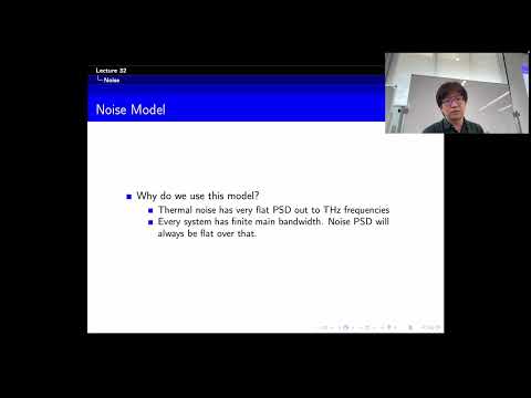
- White noise has constant power spectral density N0/2 across frequency; an ideal flat spectrum implies infinite total power.
- The infinite-power result is an idealization: practical thermal noise is approximately flat over a finite bandwidth, and channel filtering limits received bandwidth.
- A constant noise PSD corresponds to a delta-shaped autocorrelation function, with the zero-delay value representing the idealized infinite power.
- A Gaussian sample is described by its mean and variance; error probabilities are calculated using the Q-function after standardizing to zero mean and unit variance.
- Transmit filters, receive filters, and channels can all be modeled as linear time-invariant systems that process noise.
- Convolving a Gaussian random process with a filter impulse response produces another Gaussian random process.
- Multiplying a Gaussian process by a deterministic function and integrating it produces a Gaussian random variable.
- This closure under linear processing makes Gaussian noise mathematically tractable in receiver analysis.
- For continuous random variables, statistical independence is expressed by factorization of the joint PDF: fXY(x,y) = fX(x)fY(y).
- Uncorrelated variables have zero covariance, equivalently E[XY] = E[X]E[Y].
- Independence implies uncorrelatedness when the relevant moments exist, but the reverse implication generally fails.
- For Gaussian random variables, uncorrelatedness does imply independence because their joint distribution is determined by its first and second moments.
- An XOR example illustrates that statistical independence does not necessarily mean there is no underlying logical relationship between variables.
- Assuming zero-mean noise is practical because a receiver can remove a DC component.
- Whiteness gives zero correlation between noise values separated by any nonzero time lag.
- For Gaussian noise, those uncorrelated values are therefore statistically independent.
- The resulting independent-noise-sample property simplifies digital detection in the AWGN model.
- The AWGN channel receives a transmitted signal plus white Gaussian noise, producing the received waveform R(t).
- The central limit theorem helps explain why aggregate physical noise is often approximately Gaussian after normalization, even when its component sources have different distributions.
- The receiver demodulates R(t) to estimate the transmitted symbol, with the goal of making the estimate match the original symbol.
- The Gaussian approximation is a practical modeling choice as well as a mathematical convenience.
- The receiver computes an inner product between R(t) and a basis function f(t), integrating their product over time.
- This operation is a projection, analogous to extracting Fourier-series coefficients by correlating a signal with a Fourier basis.
- Using R(t) = sᵢ(t) + n(t), linearity separates the output into a signal projection and a noise projection.
- If the transmitted signal is treated as known and deterministic, its projection is a scalar signal term.
- The receiver's integrated noise term is a Gaussian random variable because it is a linear functional of a Gaussian random process.
- Its distribution can be fully specified by calculating its mean and variance.
- Those two quantities are the next step toward deriving the detector's decision rule and error performance.
Transcript excerpt
0:04 Okay, let's get started. So, [clears throat] yeah, that's review what we're covering in our last lecture. Okay. So, uh in the last lecture, we finished talking about the line coding and uh in particular, we focused on the PSD of um the uh a few waveforms, right? And uh then uh we talk about the detection in AWGN channel and uh in particular, we we talk about noise, right? And uh so this is what we cover in our last lecture. So, here is a spectral uh power spectral density of unipolar RZ, right? So, this is what we do there and so the the PSD looks like this and if you sketch it, you can see that this is what we got, right? So, basically here you can see that [clears throat] compared to the bipolar RZ, so the difference here is that we have a lot of
0:52 peaks here, right? There are a lot more delta function here, right? And the the the reason is that the zero crossing point is over is the multiples of 2 over TB and the delta here, I mean the distance the the the duration I mean the the the interval is 1 over TB, right? That's why we have a lot of this kind of peaks, right? So, those peaks I mean the DC component is not very helpful, right? So, waste of energy normally, but this peak could help could be helpful, right? So, we can uh take get some of the clock information from this kind of peaks, right? So, this could be useful. All right. And uh so we say okay, so uh for the Manchester code, so we leave that as a homework. So, if you did it did it, so this so basically what you do
This is the start of the transcript. Save this video free for the whole transcript, searchable and time-coded.
In this course
Related notes
Summary, takeaways, and chapters were generated by AI from the video's transcript and may contain errors. The video belongs to its creator, Mingyue Ji.