EEL4514C Communication Systems and Components, Fall 2026, Lecture 32
Overview
Mingyue Ji finishes the line-coding discussion by deriving the unipolar RZ power spectral density and showing how its spectral lines can support clock recovery. Ji then introduces binary detection over an additive-noise channel, motivates white Gaussian noise using interference and receiver thermal noise, and defines its flat two-sided PSD, impulse-shaped autocorrelation, Gaussian distribution, and Q-function tail probability.
Key takeaways
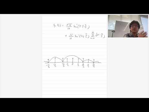
- Unipolar RZ uses a pulse lasting Tb/2, producing sinc-squared zeros at even multiples of 1/Tb while leaving spectral lines at other bit-rate harmonics that can help a receiver recover timing.
- Unipolar NRZ has a DC spectral component because its symbols are 1 and 0; unipolar RZ also has DC, but its shorter pulse changes the spectral distribution and introduces useful timing-related lines.
- An additive-noise detection model represents reception as r(t) = si(t) + n(t), with the receiver estimating the binary symbol index from the noisy waveform.
- White noise is an idealization with flat two-sided PSD N0/2; its infinite total power follows from integrating that flat spectrum over infinite bandwidth, while real receivers operate over finite bandwidth.
- The ideal white-noise autocorrelation is (N0/2)δ(τ), linking a frequency-independent PSD to zero correlation at nonzero time offsets.
- For Gaussian noise with mean μ and variance σ², a threshold-tail probability can be computed as Q((n − μ)/σ), reducing a general Gaussian probability to the standard normal tail function.
Chapters
- Midterm results are available; students can inspect exam papers in Mingyue Ji's office, and Wednesday's lecture is canceled.
- The prior lecture modeled a transmitted waveform as pulse shaping of a discrete message sequence, with output PSD determined by the pulse spectrum and the message autocorrelation.
- The line-coding analysis assumes an independent, identically distributed Bernoulli(1/2) message sequence.
- Polar NRZ maps bits to +1 and -1, while unipolar NRZ maps bits to 1 and 0 and therefore has a DC spectral component.
- Unipolar return-to-zero coding uses a pulse of duration Tb/2: a transmitted 1 produces a half-bit pulse, while 0 produces no pulse.
- Compared with unipolar NRZ, the shorter pulse changes the Fourier-transform factor to a sinc term involving Tb/2.
- The discrete-message autocorrelation stays the same as in the earlier unipolar NRZ analysis, so the new pulse spectrum supplies the key change in the output PSD.
- The half-bit pulse creates sinc-squared spectral lobes with zero crossings at 2/Tb, 4/Tb, and other even multiples of 1/Tb.
- The PSD includes discrete spectral lines spaced by 1/Tb; lines at the sinc zeros cancel, leaving components at the remaining harmonics, including odd multiples.
- The DC component remains, although it is smaller than for unipolar NRZ, and the additional lines can carry timing information.
- A receiver can extract a component at the bit rate 1/Tb to help recover clock timing.
- Ji assigns the Manchester-code PSD as practice, using the same method of finding the pulse Fourier transform and squaring its magnitude.
- The message autocorrelation can be reused from the NRZ analysis; the pulse shape is the main quantity to recompute.
- For the binary example, the two candidate transmitted waveforms are labeled s0(t) and s1(t), corresponding to the two symbol choices.
- The channel adds a time-varying noise process n(t) to the transmitted signal, producing the received waveform r(t) = si(t) + n(t).
- The receiver processes r(t) to produce an estimate î of the transmitted symbol index i.
- Because n(t) varies over time and is random, it is modeled as a random process rather than a single random variable.
- Co-channel interference can come from distant users transmitting on the same wireless channel, such as a neighbor's Wi-Fi access point.
- Adjacent-channel interference can arise from signal sidelobes; a square pulse has a sinc-shaped spectrum with sidelobes that extend beyond its main channel.
- Thermal noise remains even without other transmitters and is associated with electron motion in receiver electronics.
- Wireless received power may be around -70 dBm or lower, so comparatively small receiver noise can still impair detection.
- The detection model assumes white Gaussian noise, abbreviated WGN, with equal power spectral density at every frequency.
- The two-sided noise PSD is modeled as a constant N0/2, where N0 is determined from the noise level in the system.
- Integrating a perfectly flat PSD over infinite bandwidth gives infinite total noise power, an artifact of the idealized model rather than a finite physical receiver.
- Practical systems have finite bandwidth, and thermal-noise PSD is approximately flat over the bandwidth of interest, potentially spanning very wide frequency ranges.
- The inverse Fourier transform of the constant WGN PSD N0/2 is the impulse autocorrelation Rn(τ) = (N0/2)δ(τ), expressing zero correlation at nonzero time offsets in the ideal model.
- A Gaussian random variable is specified by its mean μ and variance σ², with variance defined as E[(N − μ)²].
- The Gaussian PDF is continuous and bell-shaped; uppercase N denotes the random variable, while lowercase n denotes a particular value or realization.
- The probability that N exceeds n is written Q((n − μ)/σ), where Q(x) is the upper-tail integral of the standard normal distribution with mean 0 and variance 1.
Transcript excerpt
0:03 Okay, let's get started. I uploaded the homework, oh no, the the result of midterm exam. And you can take a look. So let me know if you have any questions. Okay, if you don't get your exam paper, just come to my office. And yeah, I forgot to bring that today. So yeah, if you want you can you can come on Wednesday and take a look at. So normally I don't give the exam back to students. So but you can you can see where you made mistake in my office. So yeah, I think most of you did a very good job. So yeah, I didn't see any big problems. So Okay, and the other thing is that so we're not going to have lecture on Wednesday, right? And the other thing is that we'll have a Thanksgiving holiday very soon. So yeah, we're a little bit tight for
0:50 the labs. So yeah, just be you know speed up your your lab a little bit, right? So we may so I think the last lab due date would be in the reading days. So the lab will still open, yeah, but you know just prepare for that. You you may want to finish before that. Okay. Okay, so let's see what we cover in our last lecture. So in our last lecture, we talked about line coding, right? And we didn't start talking about detection of the digital signal yet, okay? So yeah, again so we focus on computing the power spectral density of the line coding, right? And here Y is the transmitted signal, right? So we model that in this
1:37 way where we have A here, right? So AK basically the function of the transmitted message. It could be either one or zero or one or minus one so on.
This is the start of the transcript. Save this video free for the whole transcript, searchable and time-coded.
In this course
Related notes
Summary, takeaways, and chapters were generated by AI from the video's transcript and may contain errors. The video belongs to its creator, Mingyue Ji.