EEL4514C Communication Systems and Components, Fall 2026, Lecture 24
 Watch on YouTube →
Overview
Mingyue Ji begins digital communications by explaining how sampling represents analog signals as discrete measurements and why digital transmission can improve noise tolerance, coding, storage, and processing. The lecture defines band-limited and time-limited signals, introduces the sampling interval and rate, and ends by modeling impulse sampling with a periodic delta train, setting up Fourier-domain analysis for the next lecture.
Key takeaways
- For regular sampling, the sampling rate and interval are reciprocals: fs = 1/Ts.
- The Nyquist sampling principle connects a signal's bandwidth to the sample rate needed for exact reconstruction, although the detailed derivation is deferred.
- A nonzero signal cannot be both absolutely limited in time and absolutely limited in frequency, a constraint that shapes practical sampling assumptions.
- Digital communication can tolerate moderate noise because receivers decide among discrete symbols, while channel coding adds redundancy to detect or correct errors.
- Impulse sampling represents each measured value as the weight of a delta impulse, enabling frequency-domain analysis that isolated point samples do not support directly.
- AMPS separates uplink and downlink with FDD, using 824 to 849 MHz for reverse channels and 869 to 894 MHz for forward channels.
Chapters
- The midterm is tentatively scheduled for Wednesday, but the usual classroom is unavailable and a second-floor room is awaiting confirmation.
- Students are asked to prepare for Wednesday; if no room is found, the exam may move to Friday or the following week.
- The previous year's practice midterm is uploaded, and this year's format and problem types are expected to be similar.
- One handwritten, double-sided cheat sheet is allowed; printed notes are not, and there is normally no class on the midterm date.
- A squaring loop removes the sign changes in the DSB-SC message, filters near twice the carrier frequency, and uses a limiter before a PLL locks to the doubled carrier phase.
- Dividing the PLL output frequency by two recovers a carrier with the appropriate phase for coherent DSB-SC demodulation.
- A Costas loop uses in-phase and quadrature branches to generate a phase-error signal and recover the message directly, rather than first recovering a carrier in a separate step.
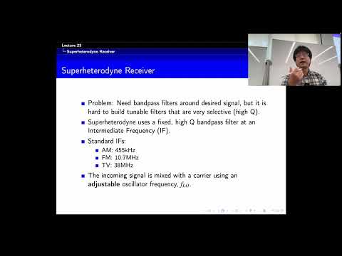
- A local oscillator mixes the received signal to a fixed intermediate frequency, where a high-Q band-pass filter can provide selective filtering.
- The lecture gives typical intermediate frequencies of about 455 kHz for AM, 10.7 MHz for FM, and 38 MHz for television.
- Mixing can also bring an image-frequency signal into the same IF band, so a tunable preselector or image-reject filter removes it before conversion.
- FM stereo combines L+R audio in the 0 to 15 kHz baseband with an L-R DSB-SC component around a 38 kHz subcarrier.
- AMPS, the first-generation analog cellular system, uses frequency-division duplexing, separating mobile-to-base and base-to-mobile frequency bands.
- The lecture gives AMPS reverse-channel frequencies of 824 to 849 MHz and forward-channel frequencies of 869 to 894 MHz.
- Cellular systems reuse frequencies in sufficiently separated cells to increase capacity while limiting interference; the lecture contrasts 2G GSM, 3G CDMA, and OFDM-based 4G.
- Sampling represents a continuous audio or video waveform by taking its value at regularly spaced time instants.
- At the receiver, recovered samples can be interpolated to reconstruct an analog waveform, but the lecture first asks when reconstruction can be exact.
- The Nyquist sampling principle is introduced as the condition under which a band-limited signal can, in theory, be recovered without loss.
- Digital receivers can decide whether a noisy observation represents a 0 or a 1, avoiding the need to reproduce every detail of the transmitted waveform.
- Shannon's channel-capacity result establishes that sufficiently low transmission rates can support arbitrarily reliable communication when suitable coding is used.
- A simple repetition-style example sends 1, 0, and their sum, adding redundancy so the original bits can still be inferred if one received value is wrong.
- Digital systems represent audio, video, and other information as bits, so a common transmitter can handle different content types instead of requiring separate analog methods.
- Error detection and correction, along with measurable bit rates, make digital links easier to analyze and manage than analog noise degradation.
- Digital information is convenient to store and process, unlike analog magnetic tapes, and digital circuits are less sensitive to component variation.
- A signal is absolutely band-limited to B when its Fourier transform is zero for all frequencies whose absolute value exceeds B.
- A signal is absolutely time-limited to T when it is zero outside the interval from -T/2 to T/2.
- A nonzero signal cannot be both absolutely time-limited and absolutely band-limited; for example, a time-limited pulse generally has frequency content extending indefinitely.
- Being unlimited in one domain does not force the signal to be limited in the other, since a signal can be unlimited in both time and frequency.
- The lecture assumes a band-limited signal with bandwidth B and samples it at regular intervals of Ts seconds.
- The sampling interval Ts is the time between consecutive samples, while the sampling rate fs counts samples per second.
- The two quantities are reciprocals: fs = 1/Ts, with units of samples per second.
- A sequence of isolated sample points cannot be analyzed by directly applying a continuous-time Fourier integral, since the point values alone have zero duration.
- Impulse sampling models the sampled signal by multiplying g(t) by a periodic delta train with impulses spaced Ts seconds apart.
- The resulting signal is a train of weighted impulses, with each impulse's weight equal to the analog signal value at its sampling instant.
- The lecture writes the sampled signal as a sum of shifted impulses and leaves its Fourier-domain analysis for the next lecture.
Transcript excerpt
0:03 All right, let's get started. Um, so hopefully you have some time to look at the lecture videos for last week. So I uploaded all of them and um and also the the lecture material including the lecture notes and slides. Okay. Yeah, I was planning to do you know to do some video. So I did two of the video before I left. I was planning to do another one during the conference but I couldn't. So I did it during the weekend. So which is this le lecture 23. Okay. And our midterm supposedly tenatively it should be in uh on Wednesday, right? But uh it will not be in this room. So this room was booked. Yeah, that's somebody uh for midterm other midterms. So we're going to have probably another classroom in the second
0:51 floor here, but I'm waiting for the confirmation. Okay. Yeah. before they told me that this book is this room is fine but I think uh last Friday I was told that this this room was not available anymore so yeah we're going to see okay so if we cannot find a room then probably we're going to postpone our midterm but now let's say it's on Wednesday okay I uploaded the the exercise midterm which was the midterm last year okay and you can take a look and uh let me know if you have any questions okay and the midterm this year would be very similar to that one. Okay. So all the the format and the problem types would would be pretty much very similar, right? So uh and the other thing is you can bring one
1:38 uh cheat sheet. Okay. Front and back, but you have to write on it. So you cannot print. >> Yes, >> that's fine. As long as it's written by
This is the start of the transcript. Save this video free for the whole transcript, searchable and time-coded.
In this course
Related notes
Summary, takeaways, and chapters were generated by AI from the video's transcript and may contain errors. The video belongs to its creator, Mingyue Ji.