ECircuits-Lec7-2026
 Watch on YouTube →
Overview
The lecture reviews ideal op-amp behavior and feedback circuits, then clarifies when virtual ground and AC-ground assumptions apply. It derives inverting and non-inverting amplifier gains, surveys summing, difference, differentiator, and integrator circuits, and introduces the finite-gain closed-loop formula for non-ideal op-amps.
Key takeaways
- An ideal op-amp's infinite open-loop gain does not make a feedback circuit's gain infinite; resistor ratios set the closed-loop gain, such as −R2/R1 or 1 + R2/R1.
- The virtual-ground approximation requires negative feedback and a finite output; it is not valid for an open-loop or positive-feedback op-amp.
- An AC ground is any node with no signal variation, even if its DC voltage is not zero; a 2.5 V reference can be an AC ground for a 0 V to 5 V amplifier.
- Negative feedback makes the closed-loop gain less sensitive to large, device-varying open-loop gain, with the ideal limit approaching 1/β.
- A differentiator places a capacitor in series with the input and a resistor in feedback, producing gain −sRC; reversing those components yields an integrator.
- For finite op-amp gain, the closed-loop gain can be expressed as A∞/(1 + 1/(Aβ)), where A∞ is ideal system gain and Aβ is loop gain.
Chapters
- The September 4 lecture introduces non-ideal op-amps after reviewing familiar ideal-op-amp circuits.
- Homework 2 is due September 14, with the instructor recommending students revisit it after this lecture and the next.
- Lab 1 runs September 14 to 17, and students are encouraged to have their components ready.
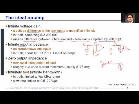
- An ideal op-amp produces Vout = A(V+ − V−), with open-loop gain A assumed infinite.
- Infinite input impedance prevents a source resistance such as Rs from forming a voltage divider that reduces the input signal.
- Zero output impedance keeps the load voltage equal to the generated output despite changes in load resistance.
- Infinite bandwidth and speed are ideal assumptions; real op-amp gain and bandwidth are finite.
- An open-loop gain of 200,000 would turn a 1 mV input difference into a theoretical 200 V output, beyond ordinary supply rails.
- Actual open-loop gain varies between devices and with voltage and temperature, so open-loop amplification is not a stable practical gain-setting method.
- Negative feedback opposes output changes; feeding the output to the inverting input reduces the V+ − V− error.
- Connecting the output directly to the inverting input creates a unity-gain buffer that can drive a load while tracking its input.
- The inverting amplifier uses input resistor R1 and feedback resistor R2, with the non-inverting input held at a reference node.
- Under negative feedback, the inverting input approximately matches the non-inverting input voltage, but the two terminals are not physically shorted.
- A ground symbol in an AC gain diagram can represent an AC ground, a node with no signal variation, rather than a node fixed at 0 V DC.
- For an amplifier powered from 0 V and 5 V, a 2.5 V DC bias can serve as an AC ground; a 0 V bias would not place the signal near the operating midpoint.
- The virtual-ground approximation applies to an op-amp with negative feedback, not to open-loop operation or positive feedback.
- With finite output voltage and ideal infinite open-loop gain, Vout = A(V+ − V−) requires the input difference to approach zero.
- Negative feedback drives that input difference toward zero by opposing the output change; positive feedback instead reinforces the change and can drive the output to a rail.
- DC bias analysis and AC signal analysis can be separated using superposition in the linear operating region.
- For the inverting circuit, the non-inverting input is an AC reference and negative feedback makes the inverting node an approximate virtual ground.
- Infinite input impedance means essentially no current enters the op-amp, so the current through R1 must also flow through R2.
- Applying KCL gives Vin/R1 = −Vout/R2, so the gain is Vout/Vin = −R2/R1.
- The negative sign indicates a 180-degree phase difference between input and output.
- With Vin applied to the non-inverting input and a divider formed by R1 and R2 on the inverting side, the gain is 1 + R2/R1.
- The feedback factor for the resistor divider is β = R1/(R1 + R2), giving ideal closed-loop gain 1/β = 1 + R2/R1.
- The feedback equation A/(1 + Aβ) approaches 1/β when open-loop gain A is very large.
- A unity-gain buffer is the non-inverting configuration with R2 shorted and R1 open, yielding gain 1 + 0/∞ = 1.
- An inverting summing amplifier combines V1 and V2 through input resistors R1 and R2, with output Vout = −RF(V1/R1 + V2/R2).
- When R1 equals R2, the summing amplifier output is proportional to the sum V1 + V2.
- Superposition provides a convenient derivation: calculate each input's contribution separately and add the outputs.
- A difference amplifier uses inputs on the inverting and non-inverting sides to produce an output proportional to their difference.
- A capacitor in the input path and a resistor in the feedback path create an inverting differentiator with gain −sRC.
- Because s = jω, differentiator gain is zero at zero frequency and increases with frequency, giving a high-pass response.
- The capacitor relation i = C·dV/dt explains the differentiator behavior in the time domain.
- Swapping the resistor and capacitor positions, with a resistor in series and a capacitor in feedback, produces an integrator and low-pass response.
- The non-ideal analysis will account first for finite open-loop gain, finite input impedance, and nonzero output impedance, with bandwidth limits treated later.
- A∞ denotes the system's ideal closed-loop gain when the op-amp open-loop gain is infinite; for a non-inverting amplifier, A∞ = 1 + R2/R1.
- For finite open-loop gain A and loop gain T = Aβ, the system gain is A∞/(1 + 1/T), equivalently A∞/(1 + 1/(Aβ)).
- The formula separates the ideal gain from its finite-loop-gain error; the lecture introduces it before continuing the detailed non-ideal analysis in the next class.
Transcript excerpt
0:00 All right. Um let's get started. Today is September 4th, lecture 7. Uh we're going to look at non ideal opamps today. But before that, we'll be also going through uh some of the basics of opamps which you already know from your other classes. And then we're going to actually delve into non ideal opamps which I believe you haven't learned in any of the previous classes. So that would be something that is completely new. uh because till now what we have learned most of these things you have learned or you have kind of uh observed this in other classes uh but we have never looked into non ideal opamps which we are going to start looking into from today's class. Now before going into that uh regarding non ideal opams um I have also uploaded homework two but homework two will be
0:48 due on September 14 so there's still uh like 10 days of time uh and by that time I think all of you will be an expert in non ideal options okay but right now if we try to look into the problems it it might seem a little bit vague and you may not understand it fully but after today's lecture and after the next lecture I think things will be much clearer question. >> Uh the first lab starts on September 14 actually right so uh I guess it's also there over here lab one and the notes required for lab one uh September 14 to 17 but I hope all of you or most of you already have your components ready all right so let's first quickly discuss
1:38 ideal opamps u something that you already know so I'll not go into the details but I'll be talking about some of the interesting facts about ideal ops
This is the start of the transcript. Save this video free for the whole transcript, searchable and time-coded.
Related notes
Summary, takeaways, and chapters were generated by AI from the video's transcript and may contain errors. The video belongs to its creator, WISE Lab - UF ECE.