ECircuits-Lec4-2026
 Watch on YouTube →
Overview
The lecture reviews Thevenin and Norton equivalents, showing how to replace a linear circuit with an equivalent source and resistance, then calculate a 50 kΩ load voltage of about 1.24 mV in a microphone example. It also introduces amplifier linearity, voltage transfer characteristics, gain, phase inversion, and DC biasing, emphasizing that useful gain requires operating in the steep region of the transfer curve.
Key takeaways
- Thevenin analysis separates a network from its load: find the open-circuit voltage, find the resistance looking into the unloaded port, then reconnect the load.
- When dependent sources are present, keep them active and use a test source to determine equivalent resistance from R_eq = V_test / I_test.
- The microphone example reduces to approximately 2.3 mV and 43 kΩ; reconnecting a 50 kΩ load yields about 1.24 mV.
- An amplifier's output energy comes from its DC supply, while its input controls the amplified AC waveform.
- Amplifier gain is the local slope of the VTC, so high gain occurs only in the steep operating region, not in the flat saturation regions.
- Biasing places the input's operating point in the high-gain region; a negative slope indicates 180-degree phase inversion.
Chapters
- Homework 1 is due Monday, August 31, and covers voltage-division and current-division problems.
- Handwritten notes for lectures 1 through 4 are available, with feedback materials posted for the next class.
- Students without a board can contact the ECE department to arrange a loan and pickup.
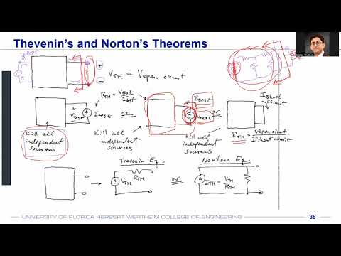
- Thevenin and Norton theorems replace a complex linear network with a single source and equivalent resistance.
- Thevenin voltage is the open-circuit voltage across the output port, where no load is connected.
- A port consists of two terminals whose currents are equal in magnitude and opposite in direction.
- To find equivalent resistance, turn off independent voltage sources by shorting them and independent current sources by opening them.
- Remove the load before measuring the resistance looking into the network from its output port.
- Apply a test voltage and calculate resistance as R_eq = V_test / I_test; dependent sources may require this method because they remain active.
- Shorting the independent voltage source makes R1 and R2 appear in parallel when viewed from the output port.
- The equivalent resistance is R1 || R2.
- The Thevenin voltage is the divider voltage across R2: V_s × R2 / (R1 + R2).
- The example microphone source is 10 mV, with R1 = 100 kΩ, R2 = 30 kΩ, R3 = 10 kΩ, and R4 = 10 kΩ.
- With the load removed and the source shorted, the output resistance is R3 + (R1 || R2) + R4, approximately 43 kΩ.
- For the open-circuit voltage, no current flows through R3 or R4; the divider across R1 and R2 gives about 2.3 mV.
- Restoring the 50 kΩ load gives a divider between 43 kΩ and 50 kΩ, producing about 1.24 mV across the load.
- Thevenin reduction gives the same result as directly solving the original network with voltage division or other circuit methods.
- Correct nodal, mesh, current-based, voltage-based, and equivalent-circuit approaches are all acceptable when they reach the correct answer.
- Thevenin and Norton equivalents require linear circuit elements, such as resistors whose voltage-current relation is V = IR.
- Diodes, BJTs, and MOSFETs are nonlinear examples, so their behavior cannot generally be represented by the same linear equivalent.
- Unilateral behavior and magnetic coupling between coils are additional cases that limit simple equivalent-circuit reductions.
- An amplifier uses energy from a DC supply to increase an AC input signal, so amplification does not violate energy conservation.
- A linear amplifier preserves the input waveform shape and ideally follows V_out = A × V_in.
- With a 5 V supply and gain of 100, an input that would demand hundreds of volts at the output clips at the supply limit and distorts into a flattened waveform.
- A voltage transfer characteristic, or VTC, plots input voltage on the x-axis against output voltage on the y-axis.
- For the common inverting response described, low input produces output near VDD, high input drives output near zero, and the transition lies between them.
- Small-signal gain is the local slope dV_out / dV_in; it is near zero on flat portions of the VTC and large in the steep transition region.
- A negative VTC slope means negative gain and a 180-degree phase inversion, not necessarily attenuation.
- An input signal centered on the steep part of the VTC can produce a larger output swing; signals in flat regions receive little gain.
- Biasing sets the amplifier's DC operating point in the high-gain region, and the course will study DC analysis before AC analysis.
Transcript excerpt
0:01 Okay. So, first off, our homework one is going to be due on Monday uh August 31st. Uh we have already discussed what is there in your homework one. It's basically a bunch of uh voltage division and current division related problems uh which we discussed in the last lecture. But let me know if there are any questions. Um I have also uploaded some of the lecture material and handwritten notes on lecture one to lecture four. Whatever we have discussed till now and what we'll be discussing today. So regarding that uh we have these handwritten notes as well. Uh on Monday we'll be also discussing a concept called feedback. So I have uploaded those lecture material as well. Uh now regarding the dad boards I know some of you had questions many of you already have the dashboards but if if anyone does not have the dboard with
0:48 you um the EC department has uh graciously agreed to uh lend the dats. For that you'll have to send an email to Mr. Eric Lener and Mr. Dan Trutor and then set up a time or schedule a time when you can pick that up from them. So if you do not have the dboard with you, uh please send an email to Mr. Lner or Mr. Trutor. All right. So today we'll be quickly
1:45 looking into the and theorem. Again most of you already know about it. This is just a very basic primer and um just a recapitulation of what you already know. Okay. uh now with Henderson Norton's theorem if you have a circuit that has many many resistors or let's say other elements as well but generally we solve those problems with registers to keep things simple uh but if you have a circuitry which has many resistors and
This is the start of the transcript. Save this video free for the whole transcript, searchable and time-coded.
Related notes
Summary, takeaways, and chapters were generated by AI from the video's transcript and may contain errors. The video belongs to its creator, WISE Lab - UF ECE.