Dynamics (MIT 16.07) - Lecture 15: Landing Rockets and Flying Cars
Overview
Jon Arrizabalaga applies the shared Newton–Euler rigid-body equations to two examples: a thrust-vector-controlled rocket landing and a Tesla Roadster stunt vehicle modeled with five cold-gas thrusters and suction. The lecture derives each system’s body-frame forces and torques, demonstrates MATLAB simulations with LQR-based controllers, and uses the rocket’s controllability matrix to show why its roll and roll rate cannot be controlled in the simplified model.
Key takeaways
- Newton–Euler equations provide a reusable rigid-body framework: the modeling challenge is specifying each system’s applied forces and torques in a consistent frame.
- A rocket with thrust magnitude T and two gimbal angles can control translation and two rotational axes, but the simplified single-engine arrangement has no roll control.
- The rocket landing demonstration uses a linearized model and LQR feedback, while the lecture describes robust rocket-landing optimization as relying on convexification to obtain guaranteed solutions.
- The flying-car force model combines four tire-contact forces, gravity, four vertical corner thrusters, one rear axial thruster, and fan-generated suction.
- The flying car’s corner thrusters provide roll and pitch moments through their lever arms, but the symmetric arrangement supplies no direct yaw authority.
- The rocket’s linearized controllability matrix has rank 10 instead of the 12 independent state dimensions, exposing the uncontrollable roll and roll-rate states.
Chapters
- Jon Arrizabalaga recaps the previous airplane model and its simulated behaviors, including stall.
- The lecture develops two new examples: a thrust-vector-controlled rocket and an unconventional flying vehicle.
- Both examples use Newton–Euler dynamics, with system-specific forces and torques supplying the main modeling work.
- The common formulation combines Newton’s law for translation with Euler’s law for rotation.
- The state includes position, orientation, velocity, and angular velocity, with the velocity quantities expressed in the body frame.
- Quadrotors, airplanes, and rockets share the same baseline equations; their applied forces and torques differ.
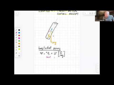
- Arrizabalaga models the rocket as a cylinder and chooses the body-frame z-axis along its longitudinal direction.
- The simplified rocket has two applied forces: engine thrust and gravity; aerodynamic drag is neglected.
- The thrust vector can be tilted by a gimbal, allowing it to generate both translation and rotational effects.
- Gravity must be transformed from the world frame into the rocket’s body frame using the orientation matrix transpose.
- The gimbal angles alpha and beta steer thrust about the body y- and x-axes, respectively.
- The three control inputs are thrust magnitude T and gimbal angles alpha and beta; together they affect translation and two rotational axes.
- The thrust vector starts aligned with the rocket, then is rotated first by alpha about the body y-axis and then by beta about the body x-axis.
- Applying the rotation matrices expresses the tilted thrust in body-frame coordinates.
- Adding the body-frame weight to the transformed thrust gives the rocket’s total longitudinal force.
- Thrust torque is calculated as the cross product of the center-of-mass-to-engine lever arm and the body-frame thrust.
- Gravity contributes no torque in this model because it acts through the center of mass.
- The gimbaled engine creates pitch and yaw authority but no roll authority; Arrizabalaga notes that real rockets can use fins and nitrogen thrusters to address rotation.
- The MATLAB model implements the derived Newton–Euler dynamics, with a shared code structure across the quadrotor, airplane, and rocket examples.
- A landing plan specifies the target location and timing, then a linearized model supplies an LQR feedback controller.
- The simulation estimates the rocket state, calculates thrust and gimbal commands, and shows the rocket landing on a pad.
- Arrizabalaga contrasts this teaching controller with more involved landing methods that seek robust, mathematically guaranteed solutions by making the optimization problem convex.
- The second example treats a Tesla Roadster stunt vehicle as a rigid body actuated by cold-gas thrusters.
- The model covers both a ramp maneuver and a flip over other vehicles, rather than ordinary road driving.
- Arrizabalaga frames the stunt as an application of Newton–Euler modeling, despite its unconventional vehicle design.
- The car’s force model contains tire forces, weight, five gas-thruster forces, and a suction force.
- Four thrusters sit near the vehicle’s corners and act along the body z-axis; a fifth rear thruster acts along the body x-axis.
- A fan-based suction system pulls the vehicle toward the ramp, helping it remain attached while upside down.
- The four wheels are numbered front-left 1, front-right 2, then rear wheels 3 and 4.
- Each tire contributes a normal force and a tangential friction force, with directions defined relative to the ramp surface.
- The four tire-force vectors are transformed into the vehicle’s body frame before being summed.
- These modeled tire forces describe road contact rather than propulsion; the simplified vehicle is driven forward by the rear thruster.
- The model omits detailed tire effects such as deformation, slip angle, and weather-dependent behavior.
- Weight is transformed into the body frame, while the five thruster forces and suction are already specified in that frame.
- The four corner thrusters contribute along body z, the rear thruster along body x, and suction acts downward along body z.
- The total body force combines tire contact, gravity, gas-thruster input, and suction.
- Each wheel’s tire force produces a torque from its lever arm relative to the center of gravity.
- The corner thrusters create roll and pitch moments, with signs determined by thruster location and the right-hand rule.
- Using lever-arm distances A and B, the roll moment is proportional to B(T1 + T4 − T2 − T3), while the pitch moment is proportional to A(T3 + T4 − T1 − T2).
- The simplified symmetric thruster arrangement provides no direct yaw torque, and centered weight and suction forces create no torque.
- The ramp and flip simulations use the same vehicle dynamics code and differ in their mission setup and controller.
- The controller remains LQR-based but adds a feedforward term, making it more involved than the rocket example.
- Plots show tire normal forces falling to zero in flight as the thrusters take over, then returning after landing.
- For the linearized rocket model, controllability is tested with the matrix formed from B, AB, and successive powers of A times B; full rank is required.
- The quaternion-based state has 13 variables but 12 independent degrees of freedom; the simplified rocket’s controllability matrix has rank 10 because roll and roll rate are unreachable.
- Zero rows in the input matrix B reveal states that direct controls cannot affect, making the missing roll authority a structural limitation of the model.
- Arrizabalaga argues that reinforcement learning depends on simulator quality and does not itself provide solution guarantees; dynamics, control theory, and numerical optimization remain essential.
Transcript excerpt
0:01 Um, welcome. Today we'll be doing cool things. Uh, I hope it's going to be a bit more fun than last time. Specifically, we'll start with a small rocket, so we'll simulate a rocket landing, and then we'll move on into let's call it an unconventional vehicle, which I'll leave for later. Um, so what did we do last time? Last time we did a small recap of all the content, and after the recap we talked a little bit on how to model an airplane. And after we modeled the airplane, we got the equations of motion, we kind of did a small simulation, and we showed some interesting phenomena like stalling and in a study. So just to refresh that, let me write it down.
0:54 Last time recap example, we saw the airplane example, and then we did a simulation of the airplanes. We kind of visualized different different behaviors. So today, as I was saying, we'll do two examples. The first example it's going to be a rocket landing. And the second example it's going to be
1:43 an unconventional aircraft. Um, okay. So maybe to break the ice a little bit. Last time we did an airplane and I was talking to Zach and we thought that half of you probably will be iron nerds and the other half will be space nerds. So who here considers himself or herself to be an space nerd? Iron nerd? Okay, so hopefully you will have fun for all both groups today, okay?
2:32 So before we start with the rocket, we have to remember one thing that all these equations have got like a common formulation, right? We take that common formulation and then we tailor the specific details of the formulation. So can someone tell me which is that common
This is the start of the transcript. Save this video free for the whole transcript, searchable and time-coded.
In this course
Related notes
Summary, takeaways, and chapters were generated by AI from the video's transcript and may contain errors. The video belongs to its creator, MIT Robotic Exploration Lab.