Dynamics (MIT 16.07) - Lecture 18: ECI Frame, Orbital Elements, and Vis-Viva Equation
Overview
Zac Manchester explains how Earth-centered inertial coordinates relate to classical orbital elements, then derives orbital period and the vis-viva equation from two-body energy and motion. He shows how to convert an ECI position-velocity state into orbital elements, highlights the singularities that make classical elements unsuitable for many numerical simulations, and applies the equations to geostationary orbit, whose semimajor axis is about 42,164 km.
Key takeaways
- ECI is centered at Earth's center of mass and fixed relative to the stars, but it is only approximately inertial because Earth accelerates around the Sun; that correction is usually negligible outside very high-precision propagation.
- The classical elements a, e, i, Ω, ω, and ν communicate orbit geometry effectively, but Ω becomes undefined at zero inclination and ω and ν lose their periapsis reference at zero eccentricity.
- For an ideal two-body orbit, period depends only on semimajor axis and gravitational parameter: T = 2π√(a³/μ), even when the orbit is elliptical.
- Matching a sidereal period of about 86,164 seconds produces a geostationary orbit with semimajor axis near 42,164 km, or approximately 6.6 Earth radii.
- The vis-viva equation v = √[μ(2/r − 1/a)] gives orbital speed magnitude at any radius without requiring a time-dependent orbit solution, making it useful for estimating maneuver Δv.
- A Cartesian state converts to orbit size and shape through ε = v²/2 − μ/r, a = −μ/(2ε), h = r × v, and e = |(v × h)/μ − r̂|.
Chapters
- The two-body problem conserves angular momentum, total energy, and the eccentricity vector.
- Classical orbital elements offer geometric intuition but have singularities related to their angle-based definitions.
- The lecture covers the ECI frame, orbital period, vis-viva speed, and conversion between state vectors and elements.
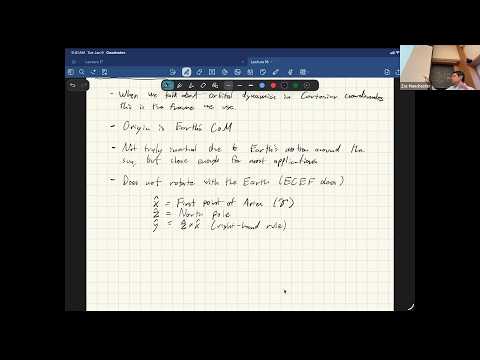
- Earth-centered inertial coordinates place the origin at Earth's center of mass and are the usual frame for satellite position and velocity vectors.
- ECI is not truly inertial because its origin accelerates as Earth orbits the Sun, but that acceleration is negligible for most applications.
- For high-precision planetary coordinates and frame conversions, JPL Horizons provides established data and software tools.
- The ECI x-axis points toward the first point of Aries, the vernal equinox direction; the name remains although the direction has shifted from the constellation Aries.
- The z-axis follows the geographic North Pole, and the y-axis completes the right-handed frame with z cross x.
- Earth-centered Earth-fixed coordinates rotate with Earth, unlike ECI; precise transformations account for wobble and other effects, so the chosen frame convention matters.
- The six elements are semimajor axis a, eccentricity e, inclination i, longitude of the ascending node Ω, argument of periapsis ω, and true anomaly ν.
- Semimajor axis describes orbit size, eccentricity describes shape, and inclination, Ω, and ω orient the orbital plane and periapsis.
- True anomaly specifies the satellite's location from periapsis; the six values encode the same state information as a 3D position and velocity.
- The eccentricity vector points toward periapsis, while the angular momentum vector h is normal to the orbital plane under the right-hand rule.
- Inclination is the angle between h and the ECI z-axis; the ascending node lies where the orbital plane crosses the equatorial plane.
- The position vector r locates the satellite, and the nodal direction provides a reference for measuring Ω and ω.
- Classical elements make orbit geometry easy to sketch and support quick, approximate mission calculations.
- In an ideal two-body model, the elements other than true anomaly are constant; real effects include nonspherical gravity, lunar and solar gravity, atmospheric drag, and solar radiation pressure.
- Perturbed elements vary over time and are called osculating elements; their evolution can be described by Gauss's perturbation equations.
- At zero inclination, the ascending node is undefined, so Ω and node-referenced angles become ambiguous and numerically sensitive near equatorial orbits.
- At zero eccentricity, periapsis has no unique direction, making ω and periapsis-referenced true anomaly undefined.
- For high-fidelity propagation and control, Cartesian state vectors are generally more robust; Cartesian gravity equations can also become numerically difficult during close approaches as the force scales with 1/r².
- For a circular orbit of radius a, the radial equation gives angular rate θ̇ = √(μ/a³), where μ is the central body's gravitational parameter.
- Dividing a full revolution, 2π, by that rate gives T = 2π√(a³/μ).
- Although derived using a circular orbit, the same period formula applies to an elliptical two-body orbit when a is its semimajor axis.
- A geostationary orbit is circular and equatorial, with a period matching Earth's rotation so the satellite stays above the same ground location.
- The relevant period is a sidereal day, 23 hours 56 minutes 4 seconds, or about 86,164 seconds, not the 24-hour solar day.
- Using the period formula gives a geostationary semimajor axis of approximately 42,164 km, about 6.6 Earth radii; communications satellites use this valuable orbital region.
- Specific mechanical energy is ε = v²/2 − μ/r; for an elliptical two-body orbit it is ε = −μ/(2a).
- Combining those relations yields the vis-viva equation, v = √[μ(2/r − 1/a)], which gives speed magnitude from orbital radius and semimajor axis.
- The equation gives no velocity direction, but it supports quick estimates of maneuver Δv when comparing speeds on different trajectories.
- Given position r and velocity v, compute specific energy ε = v²/2 − μ/|r| and then a = −μ/(2ε).
- Compute angular momentum h = r × v, then eccentricity vector e = (v × h)/μ − r̂; its norm is the scalar eccentricity.
- These calculations extract orbit size and shape directly from a Cartesian ECI state without solving the orbit over time.
- Inclination follows from the angle between h and the ECI z-axis: i = arccos(hz/|h|).
- Orbits with 0° < i < 90° are prograde, while those with 90° < i < 180° are retrograde; launching retrograde costs more because it must counter Earth's rotational velocity.
- A near-polar sun-synchronous orbit uses J2-driven nodal precession, typically slightly retrograde, to keep a consistent local solar time and lighting for Earth imaging.
- The unit nodal vector points toward the ascending node and is obtained by normalizing ẑ × h.
- Ω is measured from the ECI x-axis to the node, ω from the node to the eccentricity vector, and ν from the eccentricity vector to the position direction.
- Dot products and inverse cosine give the basic angles, while sign checks or atan2-style calculations resolve the correct quadrant over the 0° to 360° range.
- The polar equation r = h²/μ ÷ (1 + e cos ν) describes distance around an elliptical orbit as a function of true anomaly.
- At periapsis and apoapsis, the distances are rp = a(1 − e) and ra = a(1 + e), respectively.
- The semimajor axis is the average of the two apsis distances, a = (rp + ra)/2, and eccentricity can be recovered as e = 1 − rp/a or e = ra/a − 1.
Transcript excerpt
0:00 So last time what did we talk about? Um we did we talked about conserved quantities in the two body problem and this was basically angular momentum vector the total energy right kinetic plus potential. And then the third one was this weird vector that we call the eccentricity vector which um physicists like to write in a weird dimensional way and call the lelass runa lens vector even though none of those three people invented it. That's why we don't call it that. Plus the non-dimensional version is better. Um so we talked about that stuff. The the eentricity vector actually useful. We're going to use it today. Um and then we did orbital
0:48 elements. and kind of went through the the classical orbital elements. Um, fair warning, you'll see a bunch of versions of those things. Um, the reason there are so many versions of those things is because they have issues. And we'll talk a little bit about the issues today. Um and the the many the proliferation of versions and conventions of those things all has its roots in the fact that the normal sort of default set that we talked about which are the classical orbital elements have a bunch of singularities and things where they're illdefined and blow up and stuff like this. At the end of the day this is rooted in the fact that they're basically three of those orbital elements or essentially a set of oiler angles. So they have the usual oiler angle badness associated with them. So people have come up with lots of alternatives. I would argue the easiest, most straightforward alternative is if you're doing anything real involving
1:35 like high accuracy propagation or whatever, just don't use them. Just use cartigiancape vectors. Um, they're really only good for kind of like
This is the start of the transcript. Save this video free for the whole transcript, searchable and time-coded.
In this course
Related notes
Summary, takeaways, and chapters were generated by AI from the video's transcript and may contain errors. The video belongs to its creator, MIT Robotic Exploration Lab.