Dynamics (MIT 16.07) - Lecture 7: Rigid Bodies and Inertia Matrices
Overview
Zac Manchester connects rotating-frame dynamics to rigid-body mechanics, first showing how a MEMS gyroscope uses Coriolis coupling to infer rotation rate and why its simplified model is reasonable when the oscillator runs near 20 kHz. He then defines when rigid-body models are useful, represents pose with translation and rotation, and derives rigid-body kinetic energy as separate translational and rotational terms, with the rotational term governed by the inertia matrix J.
Key takeaways
- A MEMS gyro measures rotation by driving an x-axis resonator and detecting the Coriolis-induced y-axis motion, which is proportional to angular rate; phase is required to determine the rate’s sign.
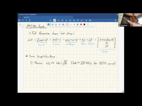
- For MEMS devices with resonances near 20 kHz, typical rotation rates of a few radians per second are sufficiently slower to justify dropping omega-squared and angular-acceleration terms in the simplified gyro model.
- A rigid-body approximation is reliable when the frequencies of flexible modes exceed the motion and control frequencies of interest; rocket bending modes around 1 to 10 Hz can overlap gimbal-controller bandwidth near 10 Hz.
- Choosing the body-frame origin at the center of mass makes the mass-weighted sum of particle positions zero and removes the cross term between translation and rotation in kinetic energy.
- Rigid-body kinetic energy separates into one-half M v-transpose-v and one-half omega-transpose J omega, with J encoding the mass distribution in the chosen body frame.
- The inertia matrix is coordinate-dependent even though kinetic energy is not, so angular velocity and J must be transformed into compatible frames.
Chapters
- The lecture revisits rotation-matrix kinematics, velocity transport, and fictitious forces: Coriolis, centrifugal, and transverse Euler terms.
- Zac Manchester previews a MEMS gyro simulation, rigid-body transformations, kinetic energy, and the inertia matrix.
- Rigid-body dynamics is framed as foundational for aircraft, launch vehicles, spacecraft, drones, and robots.
- The rotating-frame oscillator equation includes Coriolis, transverse Euler, centrifugal, spring, damping, and drive-force terms.
- For a planar chip, the model keeps x-y motion and measures angular velocity about the z-axis, normal to the chip.
- A MEMS resonant frequency around 20 kHz is far above typical vehicle rotation rates of a few radians per second, supporting the small-rate approximation.
- Small angular-rate and angular-acceleration terms justify dropping centrifugal terms proportional to omega squared and transverse terms proportional to omega-dot.
- The reduced x-y equations contain damped oscillators coupled by a 2D skew-symmetric Coriolis matrix, equivalent to a 90-degree rotation up to scale.
- Driving the x-axis strongly at resonance makes its motion predictable and lets the y-axis response act as a Coriolis signal.
- The y-axis displacement is proportional to the z-axis rotation rate, so measuring its response relative to the known x-axis drive estimates omega-z.
- The signal’s phase as well as its amplitude is needed to distinguish positive from negative rotation; in-phase and quadrature demodulation can recover both.
- With zero rotation, the simulated x oscillator builds to steady motion while the y displacement remains zero.
- A constant rotation rate produces y-axis oscillations proportional to the rate; a ramp from negative to positive rates shows an amplitude change and phase flip at zero.
- Driving at resonance boosts sensitivity, but manufacturing mismatch between x and y stiffness or natural frequency creates practical problems.
- Low damping can improve response bandwidth, while excessive drive risks mechanical nonlinearities; strong drive helps the desired signal dominate other effects.
- Mathematically, a rigid body is a collection of point masses whose pairwise distances remain constant over time, meaning it has no deformation.
- Real structures are flexible, so treating one as rigid is an engineering approximation rather than a literal description.
- The approximation is useful when flexible-mode frequencies are much higher than the frequencies of the motion, disturbances, and control actions being modeled.
- If a controller excites a flexible mode, rigid-body assumptions can fail and the structure can become unstable or suffer damage.
- Launch-vehicle bending modes can lie around 1 to 10 Hz, overlapping the roughly 10 Hz bandwidth of a gimbaled rocket motor.
- Notch filters reduce controller activity near structural resonances; trajectory planners can still use rigid-body models at slower timescales.
- Fast spacecraft pointing can excite solar-panel flex and produce settling; controllers may filter resonances or model modes to anticipate and suppress ringing.
- A highway car can often be modeled as rigid, while aggressive race-car maneuvers require attention to suspension oscillation and body roll.
- Rigid-body models are used for aircraft, spacecraft, launch vehicles, underwater vehicles, drones, and robotic systems.
- Quadruped controllers can approximate the robot as one rigid body and treat leg forces like thruster inputs.
- Configuration, or pose in robotics terminology, describes where a system is; state also includes velocity.
- A particle needs only a position, whereas a rigid body’s pose includes both position and orientation.
- Tracking every particle position is inefficient because the body’s pairwise distance constraints already tie those positions together.
- The useful configuration changes are the transformations that preserve all relative distances between particles.
- Applying a common translation vector to every particle leaves pairwise differences unchanged.
- Applying a rotation matrix also preserves distances because an orthogonal matrix satisfies Q-transpose Q equals the identity.
- A rigid body’s pose can be specified by one translation and one 3D rotation rather than by the positions of all its particles.
- Manchester denotes the rotation matrix by Q and identifies it as an element of SO(3), the special orthogonal group in three dimensions.
- The combined translation-and-rotation operation is a rigid-body transformation; robotics often represents it with a 4-by-4 homogeneous transformation matrix.
- The pose representation removes the need to track the body’s many internal distance constraints explicitly.
- The starting point is particle kinetic energy, one-half m times velocity squared, summed over every particle in the body.
- Each particle’s inertial position is written as Q times its constant body-frame position plus the body translation.
- The body frame moves with the rigid body, so each particle’s coordinates in that frame remain constant.
- Differentiating gives each particle’s inertial velocity as the body translation velocity plus the rotational contribution.
- The lecture uses Q-dot equals Q times the skew-symmetric cross-product matrix of body-frame angular velocity.
- In the stated notation, Q maps body-frame vectors to the inertial frame, while angular velocity is expressed in the body frame.
- The particle velocity becomes Q times omega-cross-r in body coordinates plus the inertial translation velocity.
- Substituting this expression into the particle-energy sum produces translation, cross, and rotation terms.
- The pure translation term sums to one-half M v-transpose-v, where M is the total mass, matching a point mass moving with the body.
- The cross term contains the mass-weighted sum of body-frame particle positions, which is the center of mass.
- Choosing the body-frame origin at the center of mass makes that weighted sum zero and removes the translation-rotation cross term.
- Using a frame not centered at the center of mass introduces extra coupling terms; link frames used in Denavit-Hartenberg robotics conventions are one example.
- The rotational energy term can be rearranged to place angular velocity on both sides of a matrix that depends on the mass distribution.
- The cross-product matrix S(r) satisfies S(r)-transpose equals negative S(r), yielding the particle contribution based on negative S(r) squared.
- Summing over particles defines the inertia matrix J as the rigid body’s rotational mass matrix.
- In equivalent form, J is the sum over particles of m times ((r-transpose r)I minus r r-transpose), using body-frame positions.
- With the body frame at the center of mass, total kinetic energy is one-half M v-transpose-v plus one-half omega-transpose J omega.
- The first term is translational energy and the second is rotational energy; they are decoupled in this representation.
- J is constant when expressed in the chosen body frame because the particle coordinates there are constant.
- The numerical entries of J depend on the coordinate frame, so J and angular velocity must be expressed in compatible frames.
- Mass is a scalar and remains unchanged by a coordinate transformation, whereas the inertia matrix’s entries change with the selected frame.
- If angular velocity is transformed by a matrix, the inertia matrix transforms by the corresponding matrix sandwich so the rotational energy remains invariant.
- The key result is a compact rigid-body energy model: total mass governs translation, while J captures how mass is distributed around the body-frame origin.
- Manchester closes by emphasizing frame compatibility when using J and omega in rigid-body equations.
Transcript excerpt
0:01 Last time we did a whole bunch of stuff about rotating reference frames, which I'd say is like quite a it's a pretty important thing. It's pretty useful. Um, we talked about rotation matrices a little bit and specifically like this kind of rotation matrix kinematic stuff, right? like how to integrate your gyro to go from omega to R dot to R basically which we'll we'll talk more about that too when we get into attitude and rigid body stuff which we're going to start today. Um then we do this like thing I called the velocity transport uh theorem which basically tells you how
0:50 velocity vectors map back and forth between a rotating and inertial frame. Um and then we sort of derived you know F= MA for the ant kind of thing and got these things we called fictitious forces and those were like your um corololis uh centrifugal and and like transverse oiler terms right that show up in the OD that come from the rotating frame and these are all like familiar things you have felt before right on like amusement park rides and cars and stuff just giving them names Um, and then the last thing we did was kind of derive this MEMS's gyro um, dynamics, kind of explain how the sensors work. So, today we're going to start back up there just so I can
1:41 hopefully like talk about that stuff a little bit more because we were running short on time last time. And I'll show you the actual simulation and what it looks like in practice. and also kind of show you that the like approximations we made with dropping a whole bunch of terms actually are valid because I'll show you the full nonlinear equations and I'll show you the one we did with
This is the start of the transcript. Save this video free for the whole transcript, searchable and time-coded.
In this course
Related notes
Summary, takeaways, and chapters were generated by AI from the video's transcript and may contain errors. The video belongs to its creator, MIT Robotic Exploration Lab.