Dynamics (MIT 16.07) - Lecture 16: Gravity, Inverse-Square Law, and The Kepler Problem
Overview
Zac Manchester develops the restricted two-body model from the inverse-square geometry of spreading light to Newtonian gravity, then uses its symmetries to explain orbital motion. He derives conservation of specific angular momentum and transforms the radial dynamics into a linear equation whose solutions give conic orbits, with eccentricity distinguishing circles, ellipses, parabolas, and hyperbolas.
Key takeaways
- An isotropic source's flux falls as 1/r² because its power spreads over a spherical surface of area 4πr²; the same geometric scaling appears in gravity and other fields.
- For spacecraft orbits, the useful measured quantity is the standard gravitational parameter μ = GM, because orbital tracking determines the product much more precisely than G or planetary mass separately.
- A central gravitational force confines motion to the plane spanned by initial position and velocity, and the absence of θ from the polar-coordinate Lagrangian makes specific angular momentum h = r²θ̇ constant.
- The nonlinear time-domain orbit equation can be converted into a linear equation for u = 1/r as a function of θ, yielding the conic equation r = (h²/μ)/(1 + e cos θ).
- Earth-orbit predictions need perturbations matched to timescale and altitude: drag is prominent below about 600 km, while J2 becomes the leading correction above that altitude and both can accumulate significant error over days.
Chapters
- The lecture shifts from prior rigid-body examples such as drones, airplanes, rockets, and flying cars to orbital mechanics.
- The restricted two-body problem models a spacecraft orbiting a much more massive planet, rather than two bodies of comparable mass.
- The goal is to connect gravity's inverse-square law to elliptical and other conic-section orbits.
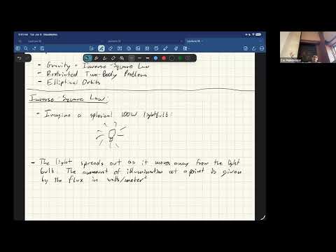
- A spherical 100-watt source spreads its power over a sphere with area 4πr².
- At 1 meter, the flux is about 8 W/m²; at 2 meters, it falls to about 2 W/m².
- The flux therefore decreases as 1/r² because the sphere's area grows with the square of its radius.
- Newton's law makes gravitational force proportional to both masses and inversely proportional to the square of their separation: F = Gm₁m₂/r².
- The gravitational constant G is approximately 6.674 × 10⁻¹¹ m³/(kg·s²).
- The same inverse-square geometry also underlies examples such as light, sound, radio waves, and Coulomb forces.
- The basic model considers only two massive bodies and ignores all other gravitational influences.
- It treats both bodies as perfect spheres, equivalently as point masses for the calculation.
- In the restricted case, the spacecraft is so much less massive than the planet that its gravitational pull back on the planet is negligible.
- Applying F = ma cancels the spacecraft mass, leaving its acceleration independent of its mass.
- The resulting point-mass equation is r̈ = −GM₁r/r³, with acceleration directed toward the planet.
- Orbital measurements determine μ = GM₁ far more accurately than G and M₁ separately; μ is known to more than 12 decimal places.
- Below roughly 600 km altitude, atmospheric drag is typically the largest correction to the point-mass gravity model.
- Earth's J2 gravity term comes from its equatorial bulge: the equatorial radius is about 30 km greater than the polar radius.
- For low Earth orbit, drag and J2 are each roughly one million times smaller than the main gravity term, but their effects accumulate over days and weeks.
- For simulations lasting only a few orbits or a few hours, the simple model may suffice; longer simulations should include drag and J2.
- Orbital elements are useful for understanding and communicating orbit geometry, but Manchester cautions against using them for real numerical simulation or controls.
- The equation r̈ = −μr/r³ is a nonlinear second-order ODE and generally does not have a direct closed-form solution for r(t).
- Symmetry and conserved quantities still reveal substantial geometric information without solving the full time history.
- Gravity always acts along the position vector r, so it cannot push the spacecraft out of the plane spanned by its initial position and velocity.
- The orbital plane is therefore fixed by the initial r and v vectors.
- Working in that plane reduces the problem to two dimensions, where polar coordinates are a natural choice.
- In polar coordinates, the kinetic energy is T = ½m(ṙ² + r²θ̇²).
- The gravitational potential energy is U = −μm/r, consistent with force being the negative gradient of potential.
- The Lagrangian L = T − U has no explicit dependence on θ, setting up a conserved angular momentum.
- The radial Euler-Lagrange equation is r̈ − rθ̇² + μ/r² = 0.
- Because θ is an ignorable coordinate, the conjugate momentum mr²θ̇ is constant.
- Dividing by spacecraft mass defines the conserved specific angular momentum h = r²θ̇.
- In three dimensions, the conserved specific angular momentum vector is h = r × v.
- In the orbital plane, a 2 × 2 skew-symmetric matrix represents a 90-degree rotation and extracts the out-of-plane component of the cross product.
- The matrix squares to −I, so its algebra resembles multiplication by the imaginary unit; the broader takeaway is that skew-symmetric matrices generalize cross-product structure.
- Instead of solving for position as a function of time, the derivation seeks the geometric curve r(θ).
- Substituting θ̇ = h/r² into the radial equation eliminates angular velocity and uses conserved angular momentum.
- The reciprocal substitution u = 1/r and a change of independent variable from time to θ make the orbit-shape problem tractable.
- After the variable changes, u(θ) satisfies a linear second-order equation with constant forcing proportional to μ/h².
- Its homogeneous solution has sine and cosine terms, while a particular solution contributes μ/h².
- Combining the solutions gives 1/r = (μ/h²)(1 + e cos θ), after choosing the angular phase so the periapsis is at θ = 0.
- Rearranging the solution gives the polar conic equation r = (h²/μ)/(1 + e cos θ).
- Eccentricity e = 0 gives a circle, while 0 < e < 1 gives an ellipse.
- The limiting case e = 1 is a parabola, and e > 1 produces a hyperbola.
Transcript excerpt
0:00 Um so last time slashl last week while I was away um John sort of dug more into uh rigid body dynamics on the kind of applied side and showed you how to handle kind of all kind of classic systems like drones, uh airplanes, um rockets and fun bonus new topic. Thank you, Elon. Uh, flying cars. Who knew? Who knew we were going to have flying cars? Uh, okay. So, that was kind of last time. And now today, we're going to start our journey into orbital mechanics. So,
0:50 first topic today is going to be gravity and in particular kind of the the inverse square law and where that comes from. Who's seen this before? Okay, just a couple of you. This is usually covered in like a freshman physics class to some degree. Um, so we'll make sure we're all on the same page there. And then we're going to from there talk about the restricted uh twobody problem [snorts] which is also known as the Kepler problem known as a bunch of things the version we're going to do here and that restricted word really refers to rather than planetary motion like earth around the
1:38 sun moon around the earth we're really focused here on spacecraft so the restricted word means that we treat one of the masses as infinite decimal um like really tiny i.e much smaller than the other mass when you're talking about the moon orbiting the earth. They're within the same order of magnitude. So that's a little different than if you have a really big planet or moon and a relatively tiny tiny spacecraft that's like many orders of magnitude lighter. So we're going to deal with that case. Um which is you know for us the the practical case. Uh
This is the start of the transcript. Save this video free for the whole transcript, searchable and time-coded.
In this course
Related notes
Summary, takeaways, and chapters were generated by AI from the video's transcript and may contain errors. The video belongs to its creator, MIT Robotic Exploration Lab.