Dynamics (MIT 16.07) - Lecture 14: Rigid-Body Systems Review and Airplane Simulation
Overview
The lecture reviews how Newton’s second law yields linear-momentum conservation and, for conservative forces, mechanical-energy conservation, then compares Newton–Euler and Euler–Lagrange methods for deriving motion equations. It applies generic body-frame rigid-body dynamics to an airplane, models aerodynamic forces and moments using dynamic pressure and coefficients, and demonstrates a MATLAB simulation with Runge–Kutta integration and an LQR controller, including low-speed and stability experiments.
Key takeaways
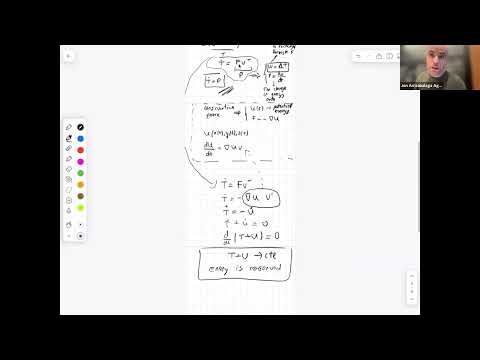
- Newton’s second law yields linear-momentum conservation when external force is zero, and for conservative forces it also yields conservation of T + U.
- Newton–Euler is convenient when external forces and torques are explicit, while Euler–Lagrange can simplify systems where internal joint forces are difficult to calculate.
- A reusable body-frame Newton–Euler model can describe different rigid bodies by changing only the force and torque models.
- Airplane lift depends on dynamic pressure q̄ = ½ρV², so reducing speed from 30 m/s to 20 m/s sharply reduces available lift and can make a demanding turn impossible.
- Center-of-gravity placement relative to the lift point determines whether disturbances produce a restoring response or amplify into instability.
- The MATLAB workflow combines nonlinear rigid-body dynamics, Runge–Kutta integration, and an LQR controller to simulate an airplane’s takeoff, route tracking, and landing.
Chapters
- The review follows the previous midterm recap, Newton–Euler derivation, and quadrotor example.
- The session is organized around a mechanics warm-up, airplane modeling, and MATLAB simulator code.
- The general law is the time derivative of linear momentum equals the net external force.
- For constant mass, momentum is mass times velocity, giving the familiar form F = ma.
- With zero external force, momentum’s derivative is zero, so linear momentum remains constant.
- For constant mass, multiplying F = m v̇ by velocity gives the rate of change of kinetic energy.
- The dot product of force and velocity is power, the rate at which force transfers energy.
- Integrating power over time gives work, which equals the change in kinetic energy.
- A conservative force is represented by the negative gradient of position-dependent potential energy: F = −∇U.
- The chain rule gives the potential-energy rate as ∇U · v, linking it to the force–velocity power term.
- Combining kinetic and potential energy rates gives d(T + U)/dt = 0, so total mechanical energy is constant.
- Newton–Euler derives motion from forces and torques, making it useful when inputs such as quadrotor rotor forces are explicit.
- Euler–Lagrange uses energy and generalized coordinates, avoiding the need to calculate many internal joint forces in complicated robots.
- Neither method is universally superior; the choice depends on system structure and which quantities are easiest to model.
- The rigid-body state includes position, quaternion orientation, body-frame linear velocity, and body-frame angular velocity.
- The control inputs are the body-frame force vector and torque vector; these enter the translational and rotational dynamics.
- The generic equations can describe a quadrotor, airplane, spacecraft, or other rigid body by changing the force and torque models.
- Body-frame modeling suits onboard systems because actuators and sensors such as an IMU measure or produce quantities locally.
- The airplane body frame uses its first axis forward, second axis lateral, and third axis upward.
- The angle of attack, α, is the angle between the forward body axis and the velocity direction.
- Sideslip angle β describes lateral misalignment of velocity; the simplified derivation sets β to zero.
- The upward body-axis convention matters because aerospace courses using a downward third axis may have different signs.
- Thrust acts along the airplane’s forward body axis, while weight points downward in the world frame and must be rotated into body coordinates.
- Drag opposes velocity and lift is perpendicular to velocity; α is used to resolve both into body-axis components.
- With β set to zero, the lateral force component is omitted; a general sideslip model would include a side force.
- The force diagram separates aerodynamic directions from the body-frame components required by Newton–Euler equations.
- The body moments L, M, and N correspond to roll about the first axis, pitch about the second, and yaw about the third.
- Ailerons, represented by δa, generate roll; elevators, δe, generate pitch; and the rudder, δr, generates yaw.
- These control-surface inputs provide the airplane’s rotational actuation, analogous to rotor-generated torques in the quadrotor model.
- Dynamic pressure is q̄ = ½ρV², where ρ is air density and V is airspeed.
- Lift, drag, and side force scale with q̄, wing area S, and their respective aerodynamic coefficients.
- Roll and yaw moments also scale with dynamic pressure, wing area, and wingspan; pitch moment uses a characteristic chord length.
- The geometric force and moment equations become predictive only once their aerodynamic coefficients are specified.
- The longitudinal coefficients are CL, CD, and CY; the rotational coefficients are Cl, Cm, and Cn.
- The lecture links coefficient dependencies to angle of attack, body angular velocity, and control deflections such as elevator, aileron, and rudder.
- The simplified dependencies are intended for conventional, low-speed flight, not aggressive fighter-jet maneuvers.
- Reliable coefficient identification is a specialized, high-fidelity aerospace modeling problem, so the simulation assumes coefficient models are available.
- The MATLAB implementation adapts the previous quadrotor code and defines mass, inertia, gravity, airplane geometry, aerodynamic coefficients, and actuator limits.
- A planned flight takes off from a runway, follows a circular route, and returns to land.
- The nonlinear dynamics are linearized about the trajectory to obtain A and B matrices for an LQR controller.
- The controller’s thrust and control-surface commands feed a Runge–Kutta integrator, which advances the airplane state and produces trajectory and input plots.
- The nominal MATLAB run uses the derived rigid-body dynamics, a Runge–Kutta integrator, and an LQR tracking controller.
- The airplane takes off, follows the red reference trajectory, circles back, and lands.
- Plots show reference versus actual position, trajectory, angle of attack, lift coefficient, thrust, and control inputs.
- Spiky actuator commands can be reduced by increasing the LQR input penalty R.
- The simulation lowers cruise speed from 30 m/s to 20 m/s while keeping the airplane, trajectory, and controller unchanged.
- Because q̄ and aerodynamic lift scale with V², the slower airplane has substantially less lift available for the same demanding turn.
- The lift coefficient falls beyond its maximum effective capacity, the airplane loses altitude, and the maneuver fails to maintain the planned path.
- With the controller removed, a nominal airplane can glide while drifting away from the reference trajectory.
- The stability experiment flips the sign of a coefficient to move the center of gravity behind the lift point.
- With the center of gravity ahead of the lift point, a wind disturbance can produce a restoring response; placing it behind the lift point amplifies the disturbance and causes the airplane to flip.
- The example connects passive stability to center-of-gravity placement and to the behavior of a linearized system.
Transcript excerpt
0:00 Okay, so with that, let's get started. Um, so what did we what do you guys do last time? I was here, so I know what you guys did. I also checked the YouTube video. Um, and I remember that you did a midterm recap. Midterm recap. Then you derived the Newton Oiler dynamics in the general sense. And finally, you moved on to the quadr example. So Newton dynamics and then the quadr today we will do it's going to be the following we'll have three steps so today we will do a warmup
0:49 warm up and as I was saying this warm-up is nothing else than kind of another recap so another recap Um then we'll move on to modeling an airplane. Okay, airplane example. And finally we will have some fun with with some simulator code in MATLAB. So simulator. Okay. So, let's get started with a recap. Um, my goal here is to kind of create a
1:40 story and to arrive to the equations of motion which we will use in the airplane. Okay. So, it's going to be maybe boring but let's let's try to follow. So, I think you studied the course with Newton's law. uh Newton's famous three laws. So, and today kind of I will put the focus on the second law. So, someone can someone tell me what's the second law of Newton? >> Yep. >> Okay. That's what I was expecting you to tell me. There is a more general form for that equation. Correct. Basically the derivative of the linear momentum is equal to correct and the momentum basically it's the mass
2:28 multiply the velocity. Awesome. Great. This is also known as the fundamental law or balance of momentum. fundamental balance of linear momentum. Okay, great. Um, now my idea here was to
This is the start of the transcript. Save this video free for the whole transcript, searchable and time-coded.
In this course
Related notes
Summary, takeaways, and chapters were generated by AI from the video's transcript and may contain errors. The video belongs to its creator, MIT Robotic Exploration Lab.