Applied Probability - F26 - Lecture 9

Overview

Arash Amini connects independence to product measures, showing how joint distributions and expectations factorize and how different couplings can share the same marginals. He then defines conditional expectation as the best mean-square prediction in an L2 space, interpreting it as an orthogonal projection onto functions measurable with respect to observed information.

Key takeaways

Independence makes the joint distribution a product measure, which is why expectations of integrable products h(X)g(Y) factor into separate expectations.
Marginal distributions do not determine dependence: independent Uniform(0,1) variables and the pair (U,U) have identical uniform marginals but different joint laws.
The L2-optimal constant estimate of X is E[X], and its minimum squared prediction error is Var(X).
Conditional expectation E[X | Y] is the mean-square-optimal prediction among functions of Y, with existence guaranteed by projection onto a closed subspace of the Hilbert space L2.
For finite-valued Y, conditional expectation is constant on each level set {Y = yᵢ} and equals E[X 1({Y = yᵢ})] / P(Y = yᵢ) when that event has positive probability.
The conditional-expectation residual is orthogonal, and therefore uncorrelated, with every square-integrable quantity measurable under the conditioning sigma field; this does not imply independence.

Chapters

0:00 Independence, Product Measures, and Joint Distributions

Independence of random variables is defined through independence of their generated sigma fields.
The joint distribution of independent variables equals the product of their marginal distributions.
For real-valued variables, independence is equivalent to factorization of the joint CDF into marginal CDFs.

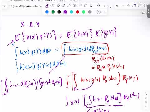
3:00 Factoring Expectations with Independent Variables

For independent X and Y, the expectation of h(X)g(Y) factors into the product of the two expectations when the integrability conditions hold.
The proof uses the joint law PXY = PX × PY, then applies Fubini or Tonelli to separate the integrals.
Without independence, the joint distribution is still needed, and the expectation generally does not factor.

6:00 Tonelli, Fubini, and the Simple-Function Proof

Tonelli applies to nonnegative measurable functions without requiring a finite integral; Fubini handles integrable signed functions.
For signed functions, check integrability of the absolute value to avoid undefined infinity-minus-infinity expressions.
The factorization identity can also be established for indicator functions, extended to simple functions, and then generalized using the Monotone Convergence Theorem.

11:00 Indicators and Independence as a Factorization Rule

Taking h and g to be indicators of events reduces the expectation identity to the defining equation P(X ∈ A, Y ∈ B) = P(X ∈ A)P(Y ∈ B).
Linearity extends the indicator case to finite sums, while simple-function approximation extends it to measurable functions.
This proof route derives expectation factorization directly from event independence.

13:14 Couplings: Same Marginals, Different Dependence

A coupling is any joint distribution with specified marginal distributions; the product measure is the independent coupling.
Two independent Uniform(0,1) variables have a uniform joint density over the unit square.
If U is Uniform(0,1) and V = U, both marginals remain uniform, but the joint law lies on the diagonal and reveals V completely once U is known.

20:00 L2 Geometry and the Goal of Conditional Prediction

Amini frames prediction of X from an observation Y as choosing a function of Y that minimizes mean squared error.
For square-integrable random variables, the inner product is E[UV], and the induced norm is the square root of E[U²].
The Cauchy-Schwarz inequality makes the inner product well-defined and gives L2 random variables a vector-space geometry.

24:00 Inner Products, Angles, and Orthogonality in L2

The L2 inner product E[UV] plays the role of the coordinate dot product used for vectors in R² or Rⁿ.
The norm of U is √E[U²], and inner products define angles and orthogonality between random variables.
L2 geometry supports the projection argument that will characterize the best prediction.

29:00 The Mean Is the Best Constant Prediction

Among constant predictions c, minimizing E[(X − c)²] gives c = E[X].
Adding and subtracting E[X] decomposes the squared error into Var(X) + (E[X] − c)².
The minimum mean-square prediction error is Var(X), the fluctuation remaining around the mean.

35:00 The Mean as a Projection onto Constant Functions

Constant random variables form a one-dimensional subspace of L2, spanned by the constant function 1.
The prediction E[X] is the projection of X onto that subspace because the residual X − E[X] is orthogonal to 1.
Orthogonality reproduces the condition that the residual has expectation zero.

38:00 Conditional Expectation as the Best Function of Y

For a general observation Y, candidate predictions are square-integrable functions g(Y).
The conditional expectation E[X | Y] is defined as the function of Y that minimizes E[(X − g(Y))²].
The minimizer exists because L2 is a Hilbert space and the subspace of square-integrable functions of Y is closed.

44:00 Fair-Die Example: Predicting a Roll from Its Parity

For a fair die, let X be the roll and let Y indicate whether X is odd.
When Y indicates odd, the best prediction is 3, the average of 1, 3, and 5; when it indicates even, the prediction is 4.
The residuals within each parity group sum to zero, illustrating the projection's orthogonality condition.

53:00 Finite Observations Produce Probability-Weighted Averages

If Y takes finitely many values, each level set Aᵢ = {Y = yᵢ} is a region where any function of Y must be constant.
On a level set with positive probability, the optimal prediction is E[X 1(Aᵢ)] / P(Aᵢ), the average of X weighted by probability.
For the fair-die parity example, equal probabilities reduce these weighted averages to the ordinary averages 3 and 4.

1:00:00 Conditional Expectation Given a Sigma Field

A random variable measurable with respect to σ(Y) can be represented as a function of Y, linking observations to available information.
The definition generalizes to any sub-sigma-field G by projecting X onto L2(G), the square-integrable G-measurable random variables.
Conditional expectation given G is unique up to probability-zero differences, so any measurable representative is a version of the same random variable.

1:07:00 Orthogonality Characterizes the Projection

The residual R = X − E[X | G] is orthogonal to every W in L2(G), which characterizes the L2 projection.
For any other candidate Z in L2(G), the squared error decomposes as E[(X − Z)²] = E[R²] + E[(E[X | G] − Z)²].
Orthogonality means the residual is uncorrelated with every G-measurable square-integrable quantity; it does not imply independence.

Transcript excerpt

0:04 US maybe this would work. Yeah. Okay. So uh we talked about product measure and I'm not going to spend too much time and then independence of um sigma fields or sigma algebbras uh which is how probabilist kind of dep they like define independence um and then um you define independence of random variables as independence of their generated sigma fields. Okay. So independence is generally like the product of intersection of a bunch of events like factorizes. And so if you take these events from uh the sigma fields generated by the random variables that would mean the random variables are independent and we we talked about like you can you can

0:51 restrict yourself to pi systems generating these um sigma algebbras by the pi lambda theorem. This is like a good exercise. And then we saw this interesting example where if x1 up to xn are independent in the above sense their joint distribution is exactly the product measure constructed from the marginal distributions. So these are marginal distributions the distributions of individual random variables. This is the joint. So the joint is really a product measure. So independence uh kind of is like the the key um uh like um concept responding to product measures. Okay. So like the distribution of independent the joint distribution of independent random variables and then a

1:39 very use and then you can also like if you have real valued random variables uh if you look at the joint CDF that's kind of like the I hope these like these are people have seen it like elementary probability here so I'm not going to spend too much time on this is like the joint CDF if they're real valued um this is going to be enough to specify its joint distribution

This is the start of the transcript. Save this video free for the whole transcript, searchable and time-coded.

Related notes

Summary, takeaways, and chapters were generated by AI from the video's transcript and may contain errors. The video belongs to its creator, ARASH AMINI.