Applied Probability - F26 - Lecture 7
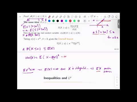 Watch on YouTube →
Overview
Arash Amini connects Lebesgue integration and expectation to practical probability bounds, deriving Markov, Chebyshev, Chernoff, and Jensen inequalities from expectation's linearity and monotonicity. The lecture then develops Lp spaces, explains how marginal and joint distributions govern moments and distances, and introduces densities, change of measure, absolute continuity, and the Radon-Nikodym theorem.
Key takeaways
- Expectation is a linear, monotone operator, so pointwise inequalities can be converted directly into probability and moment bounds.
- Markov's inequality gives P(X ≥ a) ≤ E[X]/a for nonnegative X, while applying it to squared deviations gives Chebyshev's 1/a² tail bound when variance is finite.
- A finite exponential moment E[e^(θX)] at θ > 0 yields the Chernoff bound P(X ≥ a) ≤ E[e^(θX)]e^(−θa), producing exponential rather than polynomial tail decay.
- On probability spaces, Lq is contained in Lp for q > p, and the corresponding norms satisfy ||X||p ≤ ||X||q; higher finite moments therefore guarantee lower finite moments.
- The distance E[(X − Y)²] depends on the joint distribution of X and Y, so marginal distributions alone cannot determine how close the variables are.
- A measure μ has density f with respect to ν exactly when μ is absolutely continuous with respect to ν under the theorem's sigma-finiteness conditions; then dμ = f dν and integrals transform by ∫g dμ = ∫gf dν.
Chapters
0:00
Lebesgue Expectation as Integration Against a Distribution
- The Lebesgue integral is built from indicator functions, then simple functions, then nonnegative measurable functions, and finally integrable functions.
- For a random variable X, expectation of g(X) can be computed by integrating g against the distribution, the pushforward measure of X.
- For discrete values x_i with probabilities p_i, the integral becomes the sum of g(x_i)p_i; with a density, it becomes an integral against that density.
5:00
Markov's Inequality from a Pointwise Indicator Bound
- For a nonnegative random variable X and a > 0, the pointwise inequality a times the indicator of X ≥ a is bounded above by X.
- Taking expectations preserves the inequality, and the expectation of an indicator is a probability, giving P(X ≥ a) ≤ E[X]/a.
- The bound shows that a finite first moment limits the right-tail probability at a rate of at least 1/a.
9:00
Finite Second Moments and Chebyshev's Inequality
- A finite second moment, E[X²] < ∞, ensures that X is integrable and that its variance is finite.
- Applying Markov's inequality to (X − E[X])² yields P(|X − E[X]| ≥ a) ≤ Var(X)/a².
- Chebyshev's inequality improves the generic 1/a tail bound to 1/a² when the variance exists.
16:00
Monotone Transformations Extend Markov's Inequality
- If φ is positive and nondecreasing, X ≥ a implies φ(X) ≥ φ(a), so Markov's inequality can be applied to φ(X).
- Choosing φ(x) = e^(θx) for θ > 0 produces a bound involving the exponential moment E[e^(θX)].
- The method controls one-sided tails and does not require X itself to be nonnegative.
22:00
Chernoff Bounds and Exponential Tail Decay
- The bound P(X ≥ a) ≤ E[e^(θX)]e^(−θa) follows by applying Markov's inequality to e^(θX).
- If E[e^(θ₀X)] is finite for some θ₀ > 0, setting C₀ = E[e^(θ₀X)] gives an upper bound C₀e^(−θ₀a).
- Exponential decay is faster than the 1/a decay from the first-moment Markov bound; the left tail can be treated by applying the argument to −X.
27:00
Lp Spaces Classify Finite Moments
- On a probability space, X belongs to Lp when E[|X|^p] is finite; L1 corresponds to a finite absolute first moment and L2 to a finite second moment.
- A finite higher-order moment implies lower-order moments on a probability space, so Lq is contained in Lp when p < q.
- Moment conditions also constrain tail behavior; the lecture contrasts finite moments with distributions whose moments fail to exist.
32:00
Lp Norms and the Essential Supremum
- The Lp norm is defined as (∫|f|^p dμ)^(1/p), and Lp consists of measurable functions with finite Lp norm.
- These norms satisfy properties such as the triangle inequality, allowing them to measure distances between random variables.
- For L-infinity, measure theory uses the essential supremum, which ignores changes on measure-zero sets, unlike the ordinary pointwise supremum.
37:00
Moments Describe Distributions and Norms Measure Error
- Membership of X in Lp is a condition on its distribution, obtained by integrating |x|^p against the pushforward measure of X.
- The L1 distance between X and Y corresponds to expected absolute error, while the L2 distance corresponds to mean squared error before taking its square root.
- On probability spaces, Lq norms dominate Lp norms when q > p, which gives the reverse containment Lq ⊆ Lp.
44:00
Joint Distributions Determine Distances Between Random Variables
- A pair (X, Y) maps the underlying probability space into R², inducing a joint distribution on the product space.
- The quantity E[(X − Y)²] depends on that joint distribution and cannot generally be recovered from the two marginal distributions alone.
- Different couplings can have identical marginals but different distances, such as Y = X giving zero distance versus an independent pairing.
56:00
Jensen's Inequality from Convex Supporting Lines
- For a convex function φ and integrable X, Jensen's inequality states φ(E[X]) ≤ E[φ(X)] when the terms are well-defined.
- A supporting line at m = E[X] lies below φ; substituting X and taking expectations removes the linear term because E[X − m] = 0.
- The proof uses only pointwise convexity plus expectation's monotonicity and linearity, not differentiability.
1:01:00
Jensen's Inequality Shows Lp Norm Monotonicity
- Applying Jensen's inequality to φ(x) = x² recovers nonnegative variance and shows the L1 norm is at most the L2 norm on a probability space.
- Applying Jensen to powers establishes that Lp norms increase with p on probability spaces, so higher-moment control implies lower-moment control.
- Concavity of the logarithm provides another Jensen application, illustrating how convexity and concavity yield useful expectation inequalities.
1:04:00
L2 Inner Products Preview Hilbert Space Geometry
- For X and Y in L2, E[XY] defines an inner product, while the L2 norm gives length and the inner product gives angles.
- The resulting Hilbert space structure supports geometric ideas such as projections and provides a viewpoint for conditional expectation.
- The next measure-theory topics are densities, product measures, and integration theorems including Tonelli's and Fubini's.
1:07:00
Constructing a Measure from a Density
- Given a reference measure ν and a nonnegative measurable function f, define μ(A) = ∫_A f dν for each measurable set A.
- Monotone convergence verifies countable additivity, so the construction produces a measure; the notation is also written dμ = f dν.
- The function f reweights the reference measure, assigning different contributions across the underlying space.
1:12:00
Change of Measure for Integrals
- When dμ = f dν, integrating g against μ is equivalent to integrating gf against ν: ∫g dμ = ∫gf dν.
- The identity is first checked for indicator functions, then extended to simple functions, nonnegative functions, and integrable functions.
- This provides a general change-of-measure formula rather than a rule limited to probability densities on the real line.
1:13:00
Absolute Continuity and the Radon-Nikodym Theorem
- If μ(A) = ∫_A f dν, then ν(A) = 0 implies μ(A) = 0; this relation is written μ ≪ ν and called absolute continuity.
- For suitable sigma-finite measures, the Radon-Nikodym theorem gives the converse: μ ≪ ν implies μ = fν for a nonnegative measurable density f, unique ν-almost everywhere.
- The density is denoted dμ/dν, and a proof through L2 geometry is mentioned as a later connection.
Summary, takeaways, and chapters were generated by AI from the video's transcript and may contain errors. The video belongs to its creator, ARASH AMINI.