Applied Probability - F26 - Lecture 4

Overview

Arash Amini develops the measure-theoretic foundations of random quantities: measurable maps pull target-space events back to events in the sample space, and generated sigma-algebras capture exactly the information those maps reveal. He then defines the law of a random variable as the pushforward of the underlying probability measure, illustrating the construction with finite sample spaces and explaining why a distribution is a measure rather than necessarily a density.

Key takeaways

A map X is a random variable only relative to specified sigma-algebras: every target event B must have a measurable preimage X⁻¹(B) in the source space.
To prove a real-valued function measurable, it is enough to check that {X ≤ x} is measurable for every real x, because these half-lines generate the Borel sigma-algebra.
For finite sigma-algebras, measurability is equivalent to constancy on each atom; σ(X) partitions outcomes according to the level sets of X.
If Y is measurable with respect to σ(X), then Y can be represented as g(X) for a measurable function g, expressing that Y depends only on the information revealed by X.
The joint sigma-algebra σ(X, Y) combines the information in both observations and can recover the full sample outcome when each pair of values identifies a unique outcome.
The law Pₓ is the pushforward measure defined by Pₓ(B) = P(X⁻¹(B)); unlike a density, it exists as a measure even when no density representation is available.

Chapters

0:00 Random Variables as Observable Functions of Outcomes

A random variable is a function on the sample space, which represents underlying outcomes that may not be directly observable.
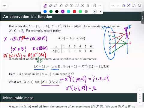
For a fair die, the indicator of an odd outcome maps 1, 3, and 5 to 1, and 2, 4, and 6 to 0.
Events about a random variable are defined by collecting the sample-space outcomes whose mapped values satisfy a condition.

6:00 Preimages Turn Real-Line Sets into Sample-Space Events

For a set B in the target space, the preimage X⁻¹(B) contains every outcome ω for which X(ω) lies in B.
Preimages are defined even when B contains values outside X's image; for the die indicator, X⁻¹((1/2, 2]) is the set of odd outcomes.
Writing P(X ∈ B) is shorthand for assigning probability to the event X⁻¹(B).

9:00 Measurability Connects Two Sigma-Algebras

A map X from (Ω, F) to (E, E) is measurable when X⁻¹(B) belongs to F for every B in E.
This condition ensures that probabilities assigned on the sample space are defined for every target-space event of interest.
For real-valued random variables, the standard target sigma-algebra is the Borel sigma-algebra on ℝ.

12:00 Generated Sigma-Algebras and Initial Measurability

Given a target sigma-algebra E, the collection {X⁻¹(B): B ∈ E} forms the smallest sigma-algebra on Ω that makes X measurable.
This is called the sigma-algebra generated by X, commonly written σ(X).
Measurability of X with respect to F is equivalent to σ(X) being contained in F.

17:00 Proving Measurability by Checking Generators

If a target sigma-algebra E is generated by a collection C, it is enough to verify X⁻¹(C) ∈ F for every C in that collection.
For a real-valued X, the half-lines (−∞, x] generate the Borel sigma-algebra, so checking {X ≤ x} ∈ F for every real x suffices.
The generator test reduces an often-large family of measurability conditions to a simpler set of checks.

22:00 Final Sigma-Algebras and the Direction of Construction

Fixing F on the source gives a largest target sigma-algebra consisting of all B for which X⁻¹(B) ∈ F.
A sigma-algebra is initial or pullback when it is the smallest one on the source making a map measurable; the final construction instead maximizes the eligible target sets.
These constructions alter the sigma-algebras used to assess measurability, not the map X itself.

27:00 Finite Sigma-Algebras: Measurability Means Constant on Atoms

When F is finite, its atoms partition Ω, and a function measurable with respect to F must be constant on each atom.
For the die's odd-even indicator, σ(X) has atoms {1, 3, 5} and {2, 4, 6}.
A finer partition may also make X measurable, but σ(X) is the smallest sigma-algebra that captures exactly the distinctions X makes.

37:00 When One Random Variable Is a Function of Another

In the finite-valued setting, Y is σ(X)-measurable exactly when Y can be expressed as a function of X.
The key is that σ(X) groups outcomes according to X's level sets, while its atoms preserve the distinct values of X.
For real-valued random variables, the corresponding factorization result says that σ(X)-measurable Y can be written Y = g(X) for a measurable real function g.

42:00 Continuous Functions and Operations Preserve Measurability

A continuous map between Euclidean spaces is Borel-measurable because the preimage of every open set is open.
Compositions of measurable maps remain measurable; since addition and multiplication on ℝ² are continuous, X + Y and XY are random variables when X and Y are.
Countable operations such as suprema, infima, limsup, and liminf also preserve measurability, sometimes yielding extended-real-valued variables.

47:00 The Sigma-Algebra Generated by Multiple Observations

For maps Xᵢ, the smallest sigma-algebra making every map measurable is generated by all their individual preimages.
For two variables, σ(X, Y) = σ(σ(X) ∪ σ(Y)); the union alone need not be a sigma-algebra, so one takes the sigma-algebra it generates.
In a finite example, the atoms of σ(X, Y) group outcomes that produce the same pair of values.

52:00 Joint Observations Combine Information

The pair (X, Y) can distinguish outcomes that neither variable identifies alone, making σ(X, Y) at least as informative as either σ(X) or σ(Y).
When each possible pair corresponds to a unique sample outcome, the joint observation determines the outcome and generates the full sample-space sigma-algebra.
The notation σ(X, Y) means the sigma-algebra generated by the maps, while σ(C) means the sigma-algebra generated by a collection of sets.

58:00 Pushforward Measures Define the Law of a Random Variable

Given a measure μ on (Ω, F) and a measurable map X into (E, E), define the pushforward by X₍ₐ₎μ(B) = μ(X⁻¹(B)).
For a probability measure P, the resulting measure Pₓ is the law or distribution of X, and Pₓ(B) equals P(X ∈ B).
P and Pₓ assign probabilities to sets in different spaces: P uses events in Ω, whereas Pₓ uses events in E.

1:05:00 Why the Pushforward Is a Valid Probability Measure

Preimages preserve complements and countable unions, so the pushforward inherits the probability measure properties from P.
In particular, the preimage of the entire target space is Ω, the preimage of the empty set is empty, and disjoint target sets have disjoint preimages.
The same construction works for a general measure μ, not only for probability measures.

1:10:00 Finite Examples: Pushing Die Probabilities onto Values

Under the uniform distribution on die outcomes 1 through 6, the odd-even indicator pushes the mass to a distribution with probability 1/2 at 0 and 1/2 at 1.
For a finite-valued map, outcomes in each level set contribute their total probability mass to the value shared by that set.
A real-valued die function with three equally likely outcomes in its level sets has a pushforward formed from three point masses of 1/3 each.

1:14:30 Distributions Are Measures; Densities Are Optional Descriptions

A distribution is fundamentally a measure assigning values to measurable sets; a density is only one possible way to represent that measure.
For continuous distributions, singleton probabilities may be zero, so listing masses at individual points—as in finite examples—does not describe the law.
Amini previews quantile transforms for constructing laws from a uniform random variable, random elements, and the later development of expectation and integration.

Summary, takeaways, and chapters were generated by AI from the video's transcript and may contain errors. The video belongs to its creator, ARASH AMINI.