Applied Probability - F26 - Lecture 12

Overview

Arash Amini develops regular conditional distributions as probability kernels, shows how they factor a joint law into a marginal and a conditional law, and connects that framework to Bayes' rule. A Gaussian prior with Gaussian observation noise yields an explicit Gaussian posterior whose mean weights the prior and observation by their precisions; the lecture then extends the posterior formula to arbitrary prior measures observed through a Gaussian channel.

Key takeaways

A regular conditional distribution is a probability kernel, and it factors a joint law into the marginal law of the conditioning variable and the conditional law of the other variable.
The kernel factorization gives a sampling recipe: draw Y from its marginal, then draw X from K(Y, ·); independence is the special case where K does not depend on Y.
With X ~ N(m, s²) and Y|X=x ~ N(x, σ²), the posterior variance is (1/s² + 1/σ²)⁻¹ and the posterior mean weights m and y according to their relative precisions.
The Gaussian posterior mean is the optimal squared-error denoiser, and its weights shift toward the observation when prior uncertainty is high and toward the prior when observation noise is high.
Bayesian updating does not require a prior density: a general prior measure μ can be combined with a likelihood density by integration, even when the resulting observation distribution is not Gaussian.

Chapters

0:00 Conditional Distributions as Probability Kernels

A regular conditional distribution K(y, B) is a probability measure in the event B and a measurable function of the conditioning value y.
A conditional law can be identified by its expectations against a sufficiently rich class of test functions.
To verify a proposed kernel, check the conditional-expectation identity, often first for indicator functions.

4:00 Bayes' Rule: Likelihood, Prior, and Posterior

For a joint density p(x,y), the conditional density is p(x|y) = p(x,y)/p(y), where p(y) is obtained by integrating out x.
Bayes' rule equates likelihood times prior with the joint density: p(y|x)p(x) = p(x,y).
For a fixed observation y, the posterior is proportional in x to p(y|x)p(x); normalization makes it integrate to one.

9:00 Deriving Joint-Law Factorization with Conditional Expectation

The probability of a rectangle event {Y in A, X in B} is the expectation of the product of its two indicator functions.
The tower property conditions first on Y, reducing the inner expectation to P(X in B|Y).
Integrating that conditional probability over A with respect to the marginal law of Y recovers the joint probability.

18:00 Writing a Joint Measure as a Marginal and a Kernel

The joint law can be written compactly as the marginal measure of Y combined with the conditional kernel K(y, dx).
On a rectangle A × B, the notation means integrating K(y, B) over y in A under the marginal law of Y.
In the density case, the same factorization becomes p(x,y) = p(x|y)p(y).

24:00 Conditional Sampling Versus Independent Product Measures

To sample from the factored joint law, first draw Y from its marginal and then draw X from K(Y, ·).
This is more general than a product measure because the conditional kernel can depend on the sampled Y.
If K does not depend on Y, the factorization reduces to independent sampling from two fixed marginal measures.

28:00 Constructing a Joint Law from Any Kernel and Marginal

A probability measure ν and a probability kernel K define a joint measure on the product space through integration of K against ν.
This construction generalizes the section-based construction of product measures and assigns the expected mass to measurable rectangles.
The required measurability and measure properties follow from a standard measurable-set argument, outlined in the lecture notes.

34:00 Gaussian Prior and Noisy Observation Model

The example starts with a prior X ~ N(m, s²) and an observation model Y|X=x ~ N(x, σ²).
The observation can be generated as Y = X + σZ, with Z standard normal and independent of X.
Here s² measures prior uncertainty, while σ² describes the observation noise.

40:00 Using Independent Gaussian Noise to Obtain a Joint Normal

Because X and Z are independent normal variables, their pair is jointly Gaussian; Y = X + σZ is a linear transformation of that pair.
The resulting marginal has Y ~ N(m, s² + σ²), since independent variances add.
The covariance calculations use Cov(X,Y) = s² and Cov(Z,Y) = σ, illustrating covariance bilinearity.

48:00 Checking the Gaussian Observation Model from the Joint Law

The joint Gaussian law of X and Y can be obtained from the mean vector and covariance matrix of the linear construction.
Using the joint density divided by the marginal density recovers Y|X=x ~ N(x, σ²).
This verifies that the additive-noise construction and the stated conditional observation model describe the same joint distribution.

52:00 Deriving the Gaussian Posterior by Bayes' Rule

For an observed value y, multiply the likelihood proportional to exp(-(y-x)²/(2σ²)) by the prior proportional to exp(-(x-m)²/(2s²)).
The product is an exponential of a quadratic in x, so completing the square identifies a Gaussian posterior.
The posterior variance is V = (1/s² + 1/σ²)⁻¹ = s²σ²/(s² + σ²), and the posterior mean is V(m/s² + y/σ²).

59:00 Interpreting Posterior Weights and Precision

The posterior mean is a weighted average: (σ²/(s² + σ²))m + (s²/(s² + σ²))y.
A large prior variance s² weakens the prior and increases the weight on observation y; a large noise variance σ² does the opposite.
Posterior precision is the sum of prior precision and observation precision, 1/V = 1/s² + 1/σ².

1:03:00 The Posterior Mean as a Gaussian Denoiser

The conditional mean E[X|Y=y] is the linear estimator d*(y) = V(m/s² + y/σ²).
For squared-error prediction, this conditional expectation is the best estimate of X given the noisy observation.
The conditional variance V is constant in y for this Gaussian model, although the conditional distribution changes with y through its mean.

1:05:00 Bayesian Updating with a General Prior Measure

The prior can be any probability measure μ; it need not have a density with respect to Lebesgue measure.
When Y|X=x has density p(y|x), the marginal observation density is obtained by integrating p(y|x) against μ(dx).
The posterior kernel combines the likelihood with μ, extending the usual density form of Bayes' rule.

1:08:00 A Gaussian Channel with an Arbitrary Input Distribution

For the Gaussian channel Y|X=x ~ N(x, σ²), the likelihood is a translated Gaussian density centered at x.
If the input prior μ is non-Gaussian, the marginal distribution of Y need not be Gaussian.
The posterior still has a density under this Gaussian likelihood; the general-measure calculation is developed further in the next lecture.

Transcript excerpt

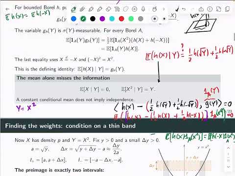
0:00 Okay, so we're talking about the and um so the idea was there is this um object which is um a probability measure in the second argument and a measurable map in the first argument and it describes basically the conditional regular conditional expectations sorry regular conditional distributions. So the meaning of like kyb is the like a probability of like x in g like in b given y is equal to y generally like describes the like the conditional relation between two random variables and then we have this general kind of existence result that you can like basically

0:47 describe this conditional distribution via uh evaluating expectations under a test function. this the idea very general we discussed this and we'll come back to it so if I if I specify the expectations of h of x for some uh function h in a large enough class uh this describes a distribution and so this is this this expectation here um being written like this is describing the conditional distribution of xq and why um we did an example um this you'll do in your homework and then we talked about this slide which is

1:34 um usually like you can guess and then verify um using this identity. So if you have a guess of a conditional distribution u like that kernel uh then if you want to prove that that's really like you're given two random variables and you have a like a guess of the kernel you try you can you can try to prove that this is indeed the conditional expectation sorry a conditional distribution if you verify this identity so this is well defined by other means by projection so you you try to figure out what is a conditional expectation of h of xq and y for a generic h and if it

This is the start of the transcript. Save this video free for the whole transcript, searchable and time-coded.

In this course

Related notes

Summary, takeaways, and chapters were generated by AI from the video's transcript and may contain errors. The video belongs to its creator, ARASH AMINI.