Applied Probability - F26 - Lecture 11

Overview

Arash Amini develops conditional expectation into the idea of a regular conditional distribution, represented by a probability kernel that assigns a probability measure to each observed value of a random variable. He illustrates the construction with X uniform on [-1,1] and Y = X², verifies the resulting two-point conditional law using symmetry and conditional-expectation orthogonality, and concludes with the density-ratio formula for joint densities.

Key takeaways

A probability kernel K(y,B) resolves the version problem in conditional probability by requiring B ↦ K(y,B) to be a probability measure for each y and y ↦ K(y,B) to be measurable for each B.
For real-valued X and Y, the regular conditional distribution represents every bounded Borel conditional expectation through E[h(X) | Y] = ∫h(x)K(Y,dx).
When X is uniform on [-1,1] and Y = X², the conditional law of X given Y = y places equal mass on √y and -√y; symmetry verifies the weights.
Matching only E[X | Y] is not enough to identify a conditional distribution; verification must use indicators or another class of functions rich enough to distinguish probability measures.
When a joint density exists, the conditional density follows from the joint-to-marginal ratio, pX|Y(x|y) = pXY(x,y)/pY(y), and the reverse conditional formula yields Bayes' rule.

Chapters

0:00 Conditional Expectation Connects Expectations to Probabilities

The L² projection view gives intuition for conditional expectation, and its useful properties extend to L¹.
For a random variable X, its distribution satisfies P(X ∈ B) = E[1_B(X)].
This indicator identity motivates defining conditional probability through E[1_B(X) | Y].

2:00 Why Conditional Expectations Need Consistent Versions

E[1_B(X) | Y] defines a random variable only up to almost-sure equality.
The exceptional null set can depend on the set B, so independently chosen versions may fail to form a probability measure as B varies.
A conditional law requires versions that fit together into one probability measure for each observed value of Y.

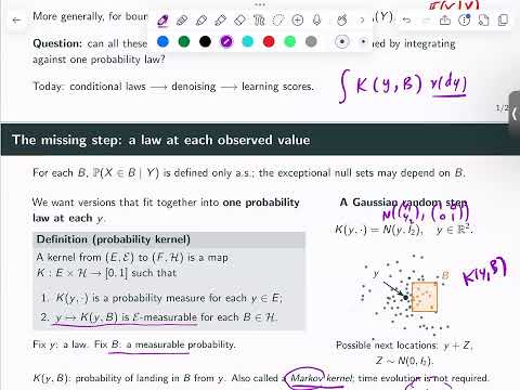
6:00 Probability Kernels Combine Measurability and Probability Measures

A probability kernel K maps an observed point y and a measurable set B to a value K(y,B) in [0,1].
For each fixed y, B ↦ K(y,B) must be a probability measure; for each fixed B, y ↦ K(y,B) must be measurable.
Probability theory also calls this object a Markov kernel, though it is distinct from similarity kernels used in machine learning.

9:00 A Gaussian Kernel Models a Random Next Step

A two-dimensional example assigns K(y, ·) a Gaussian distribution with mean y and identity covariance.
For a set B, K(y,B) is the probability that a step starting at y lands in B.
Chaining such transition kernels provides the basic construction for Markov processes.

13:00 Kernel Measurability Makes Conditional Probabilities Integrable

Fixing B makes K(·,B) a measurable, nonnegative function of the current value, so it can be integrated against another measure.
Fixing y instead makes K(y,·) a measure, allowing measurable functions to be integrated with respect to it.
A kernel can also be viewed more abstractly as a measure-valued random variable, though that viewpoint requires a sigma-field on the space of measures.

17:00 Regular Conditional Distributions Represent Conditional Expectations

For real-valued random variables X and Y, a regular conditional distribution provides a kernel K from values of Y to probability measures on values of X.
For every bounded Borel function h, E[h(X) | Y] = ∫ h(x) K(Y, dx) almost surely.
The integral is taken against the measure K(y, ·) after fixing y; boundedness ensures the integral is well-defined.

24:00 Indicators Recover Conditional Probabilities from the Kernel

Setting h(x) = 1_B(x) in the kernel formula gives E[1_B(X) | Y] = K(Y,B) almost surely.
Thus K(y,B) supplies a coherent version of P(X ∈ B | Y = y), even when the event Y = y has probability zero.
The kernel represents the whole conditional distribution, not just the conditional mean of X.

27:00 Conditional Laws Are Defined Pointwise Through a Kernel

The expression P(X ∈ B | Y = y) can be defined as K(y,B), while the corresponding random conditional probability is K(Y,B).
For each fixed y, the kernel guarantees that these probabilities across B form a measure.
This construction resolves the version-consistency issue that arises when conditional expectations are defined only almost surely.

33:00 The Kernel Formula Is a Recipe for the Projection

The kernel integral computes a random variable that is a function of Y, matching the role of the conditional-expectation projection.
The geometric projection interpretation concerns the resulting random variables; the kernel supplies a concrete integration formula for calculating them.
A single conditional mean does not determine a conditional distribution, so the formula must hold for a sufficiently rich class of functions.

36:00 Conditioning on X Squared Leaves Two Possible Signs

Let X be uniform on [-1,1] and set Y = X²; the joint values (X,Y) lie on the parabola y = x².
For an observed y in [0,1], the only possible values of X are √y and -√y.
Symmetry suggests equal conditional probabilities, giving K(y,·) = ½δ√y + ½δ−√y, up to choices on null or out-of-range values of y.

40:00 Integrating Against the Two-Point Conditional Law

For a bounded Borel function h, the proposed kernel gives ∫h(x)K(y,dx) = ½h(√y) + ½h(-√y).
Evaluating this function at the random variable Y gives ½h(√Y) + ½h(-√Y).
To establish the candidate as the conditional law, Amini uses the conditional-expectation orthogonality criterion rather than checking only one output.

46:00 Symmetry Verifies the Conditional Law for General Functions

The verification checks that the proposed conditional expectation has zero error when integrated against indicators of events in σ(Y).
Because Y = X² is unchanged when X is replaced by -X, and the uniform distribution on [-1,1] is symmetric, the two sign contributions balance.
Checking only h(x) = x would establish the conditional mean is zero, but not the full distribution; different laws can share the same mean.

55:00 Conditional-Kernel Uniqueness, Density Weights, and Bayes' Rule

A regular conditional distribution is unique up to equality of probability measures for almost every value under the distribution of Y.
For a nonsymmetric density of X, the two possible values ±√y generally receive different weights, proportional to the density near those points.
A heuristic derives weights by conditioning on a small interval around y; a rigorous approach verifies the candidate using conditional-expectation identities.
If (X,Y) has joint density pXY, the conditional density is pX|Y(x|y) = pXY(x,y)/pY(y) when pY(y) is positive, with the reverse conditional density giving the usual Bayes' rule.

Transcript excerpt

0:00 Yeah. Okay. Yes, okay. It should work now. Okay, so let's continue. We started I believe talking about So, these slides by the way are updated um multiple times now. So, if you want to grab the latest version from the box. So, um So, I want to maybe extensively talked about conditional expectation. Right? Um and there's a formal way of defining it which is via um I mean, the way we we expressed it is via the the projection idea, which is very useful. And then the L2 projection and then you can extend it to L1. There's a bit of details at the end of the PS set of slides and also the notes I

0:47 posted go going to more detail how to extend it to L1. Uh but the projection idea is very useful for intuition and for the properties. Basically, all the interesting properties of conditional expectation like the nested product power property, they are properties of projections basically that that extend to the L1 case. So, once we have the conditional expectation, um because there is a there's a link between probabilities and the expectation operator. So, if you remember um the um this P of X. So, if you have a random variable X, PX of B is the the the the basically, probability assigned to B under the law or the distribution of X, which is

1:33 equal to this or defined like this, probably the X belongs to B. And this can be written as the expectation of the indicator of B applied to X, okay? This is this is random variable takes value zero and one, takes the value one with this probability. So, it'll be one times this probability plus zero times the complementary probability. So, it would be just this probability, right?

This is the start of the transcript. Save this video free for the whole transcript, searchable and time-coded.

In this course

Related notes

Summary, takeaways, and chapters were generated by AI from the video's transcript and may contain errors. The video belongs to its creator, ARASH AMINI.