RL @ ECE-UofT - Lecture 07: Policy Evaluation via Function Approximation

Overview

Ali Bereyhi explains why tabular reinforcement learning does not scale to enormous or continuous state spaces, then develops function approximation as a way to generalize value estimates from sampled states. The lecture derives least-squares training with gradient descent, shows how Monte Carlo and TD targets train value and Q networks, and proves tabular TD is a special case of linear approximation with one-hot state features. It closes with eligibility-trace extensions, a mountain-car illustration of smoother value estimates, and a preview of deep Q-learning, policy gradients, and actor-critic methods.

Key takeaways

A tabular control method needs roughly C × N × M samples to estimate all state-action pairs, and continuous or high-dimensional state spaces make exhaustive coverage infeasible.
Function approximation learns values at sampled states and generalizes through shared parameters, allowing a single gradient update to affect many unvisited states.
For policy evaluation, least-squares training minimizes Eπ[(V̂(S; w) − Vπ(S))²], with Monte Carlo returns or one-step TD targets providing practical value estimates.
Tabular TD is a special case of gradient-based function approximation: one-hot state features and a linear value model produce a gradient that updates only the visited state's weight.
A Q network with M outputs can estimate all action values for a state and support greedy Q-learning, but this architecture requires a finite action set.
Neural value approximation produces smoother estimates than a discretized mountain-car table because updates to shared weights also affect nearby position-velocity inputs.

Chapters

0:00 From Tabular RL to Function Approximation

The course has covered model-based value and policy iteration, then model-free prediction and control.
Generalized policy iteration alternates policy evaluation with greedy policy improvement.
Monte Carlo and temporal-difference methods estimate values; SARSA is on-policy control and Q-learning is off-policy control.

3:00 Why Tabular Control Requires State-Action Coverage

A tabular Q method stores one value for each of N states and M actions, requiring N × M entries.
If each state-action pair needs C samples, a rough uniform-coverage estimate is C × N × M samples.
Actual trajectories visit states unevenly, so some table entries may remain poorly estimated or unseen.

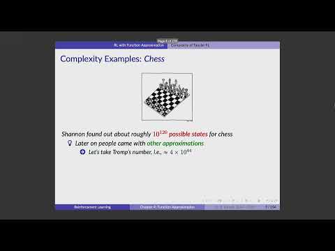
8:00 Chess Shows the Limits of a Q-Table

The lecture cites Claude Shannon's estimate of roughly 10^120 possible chess positions or game-tree possibilities.
Even assuming an extremely fast picosecond per sample and only 10 samples per pair, the example estimates about 12 × 10^25 years of computation.
That estimate dwarfs the universe's roughly 14-billion-year age, making exhaustive table construction impractical.

13:00 Continuous States Create Exponential Grid Costs

Cart-pole state includes continuous variables such as cart position and pole angle, yielding infinitely many possible states.
Discretizing L state dimensions into B bins creates B^L grid points; even modest dimensionality makes the grid grow rapidly.
Tabular methods remain mathematically valid, but state coverage makes them unusable in many practical problems.

18:00 Function Approximation Replaces State-by-State Storage

Instead of storing a value for every state, estimate values at sampled states and fit a parameterized function to them.
A neural network can then return an estimated value for states that have not yet been visited.
DeepMind's 2014 to 2015 deep Q-learning results renewed attention to neural-network function approximation.

21:30 Representing a Policy Value with a Parameterized Model

For a fixed policy π, represent its value estimate as V̂(s; w) = f(s, w), with state s as input and learnable parameters w.
A linear regression model uses weights and a bias; an MLP, CNN, or transformer can serve as a more expressive model.
Sampled states and estimated values provide training pairs for fitting the model.

28:00 How One Weight Update Generalizes Across States

Changing neural-network weights can change estimated values for many states, not only the state in the latest sample.
This shares information across nearby or structurally related states, unlike independent entries in a value table.
For cart-pole, a small change in pole angle should usually produce a nearby value estimate rather than an unrelated zero.

32:30 Neural Networks as Flexible Value-Function Models

The course focuses on linear models and neural networks as function approximators, while Fourier and wavelet features are also possible.
The universal approximation theorem motivates using sufficiently wide or deep neural networks to represent complex value functions.
The theorem guarantees representational capacity, not that training will find the ideal weights.

37:00 Training Models with Empirical Risk and Mini-Batch SGD

Training data pairs an input state x with a target value y, and empirical risk averages prediction loss across the dataset.
Full-batch gradient descent averages gradients over all samples before each update.
Mini-batch SGD uses a random batch of size B to reduce computation; its average gradient is an unbiased estimate of the full-data gradient.

45:00 State Features: One-Hot Vectors, Measurements, and Screens

A state should be encoded as a feature vector, not simply passed to a network as an arbitrary state index.
For a known finite state set, one-hot encoding represents state n with a vector whose nth entry is 1.
Continuous cart-pole states can use position and angle directly; game-playing agents can use screen frames as CNN inputs.

54:00 Mountain Car Uses Position and Velocity as Features

Mountain car can represent a state with the car's position x and velocity v, with optional measurements such as acceleration or tire friction.
The agent chooses left acceleration, right acceleration, or no acceleration to escape the valley.
The example assigns a reward of −1 per step before reaching the goal, encouraging fewer steps to the hilltop.

1:00:00 Linear and Neural Value Models for Mountain Car

A linear value model for mountain car can use two weights, one multiplying position and one multiplying velocity, plus an optional bias.
If the value function is not well represented by a linear combination, a neural network can add hidden units and layers.
The feature vector describes observed state properties; it is not necessarily the full underlying Markov state.

1:05:00 Least-Squares Loss for Policy Evaluation

The ideal training target is the true policy value Vπ(s), while the model produces V̂(s; w).
Mean squared error minimizes the squared difference between predicted and true values.
Weighting errors by the policy's state-visitation probabilities gives the objective Eπ[(V̂(S; w) − Vπ(S))²].

1:12:00 Backpropagating Value-Function Prediction Errors

Differentiating squared error produces a term proportional to (V̂(S; w) − Vπ(S)) times ∇w V̂(S; w).
A neural network computes the prediction gradient by backpropagation after a forward pass on the state.
Sampling states from policy-generated trajectories gives a Monte Carlo estimate of the expected gradient.

1:18:00 Gradient Descent Updates for Value Networks

Gradient descent updates weights by subtracting the learning rate times the estimated loss gradient.
Absorbing the factor of two from squared error into the step size yields an update proportional to the target-minus-prediction error times the network gradient.
The estimated policy value can come from Monte Carlo or TD methods rather than an unavailable exact value.

1:21:00 Monte Carlo Returns as Value-Network Targets

For a trajectory, the return Gt sums rewards from time t onward and estimates Vπ(St).
Each pair (St, Gt) can contribute a value-network gradient sample.
Averaging gradient samples over visited states naturally weights frequently encountered states more heavily under the policy.

1:25:00 A Trajectory as a Mini-Batch for Monte Carlo Learning

One episode supplies T training examples, (S0, G0) through (ST−1, GT−1).
For each state, a forward pass gives V̂(St; w), and backpropagation computes its gradient contribution.
The algorithm averages the episode's sample gradients, updates the network, then collects another trajectory.

1:30:00 Online Monte Carlo Updates Within an Episode

A complete episode can be treated as a mini-batch, but smaller batches allow more frequent updates.
Using a single state-return sample per update is stochastic gradient descent with higher gradient variance.
The update resembles tabular Monte Carlo: move the estimate toward Gt, multiplied by the value network's parameter gradient.

1:34:30 TD Targets Train Value Networks Without Full Returns

The one-step TD target for state St is Rt+1 + γV̂(St+1; w), using the network's prediction for the next state.
This bootstrapping target can update before an episode ends, unlike a full Monte Carlo return.
TD introduces bias through the current estimate, while Monte Carlo targets generally have higher variance.

1:40:30 Tabular TD Is Function Approximation with One-Hot Features

With one-hot state features and a linear model, V̂(s; w) selects the weight corresponding to that state's index.
The gradient of the predicted value with respect to all weights is the same one-hot vector.
Applying the function-approximation update therefore changes only the weight for the visited state, reproducing tabular TD.

1:45:00 Deriving the One-Hot Gradient for a State Value

For state Sn, the one-hot feature vector has a 1 at position n and zeros elsewhere.
Taking its inner product with the weight vector returns wn, the tabular value estimate for Sn.
The parameter gradient is zero for every weight except wn, where it is 1.

1:50:00 The Generalized TD Update Reduces to the Table Update

Substituting the one-hot gradient into the weight update leaves all unvisited-state weights unchanged.
The selected weight moves toward the TD target, reward plus discounted next-state value.
Tabular TD is thus a restricted case of function approximation using tokenized states and a linear model.

1:55:00 From State Values to Q Networks

A Q network estimates action values for state-action pairs, extending value approximation from Vπ(s) to Qπ(s, a).
A state-action representation can be fed into a model that returns the value for that pair.
Alternatively, a network can take only the state representation and output one value for each discrete action.

1:59:00 One Q-Network Output per Discrete Action

For a state with M possible actions, the network can produce an M-dimensional vector of action-value estimates.
The maximum output supports greedy action selection for Q-learning, while a policy can also select among the outputs.
This output design handles continuous states but assumes a finite, countable action set.

2:05:00 Why Continuous Actions Need a Different Q-Network Design

A fixed network output layer must specify its number of action values, so the described architecture does not directly support continuous actions.
A finite-action robot might choose among north, south, east, and west, which fits the M-output design.
Deep deterministic policy methods are previewed as a later approach to continuous-action control.

2:10:00 Least-Squares Training for Q Networks

Q-network training minimizes squared differences between predicted action values and target action values.
Backpropagation differentiates the selected Q output with respect to network weights.
Monte Carlo returns or TD targets can supply the action-value training target.

2:15:00 Eligibility Traces as Gradients of Action Values

Tabular TD(λ) updates eligibility traces by multiplying existing traces by γλ and adding 1 to the current state-action pair.
Under one-hot state-action features and a linear Q model, the Q-value gradient is the one-hot representation of that pair.
The trace update can be generalized by replacing the one-hot feature with the gradient of the Q network.

2:20:00 Extending Eligibility Traces to Function Approximation

In the tabular representation, the eligibility map contains one entry for each state-action pair.
A general approximate trace can accumulate discounted gradients of Q with respect to network weights.
Value networks, Q networks, policy networks, and eligibility traces can all be parameterized and trained through gradient-based updates.

2:25:00 Mountain Car Shows How Function Approximation Smooths Values

A discretized position-velocity table can look jagged because sampled cells update while neighboring cells remain at zero.
A neural network shares parameters across states, so updates at observed positions and velocities also influence nearby estimates.
The lecture previews value-based control with SARSA and Q-learning, policy-based TRPO and PPO, and actor-critic systems with policy actors and value critics.

Transcript excerpt

0:00 So, today we're going to talk about function approximation. So, it's uh like say, first chapter we get on deep reinforcement learning. Uh just a quick recap what we have done up to this point. Up to this point we have talked about tabular reinforcement learning. And within that one, we started with model-based case. In the model-based case, you essentially have the MDP, right? You do not have does the environment look like, and then based on that one, you you are able to actually define the optimal policy. You can write down the Bellman equation. That one helps you developing algorithms to find the optimal policy, right? And the two main algorithms we talked about, they

0:48 were value iteration, policy iteration, and we said they are actually uh two edges or two extreme cases of a generalized policy iteration algorithm. Uh the idea here was we always evaluate a policy, and once we have the value or approximate value for that policy, we opti- we improve by just doing greedy, right? So, that was the idea here, and then this somehow was helpful in the sense that we learn about Bellman equation, we learn about this recursive property within the reinforce- reinforcement learning setting. And that one helped us to develop approaches for doing model-free reinforcement learning. And here we assume that we don't know the MDP,

1:34 right? MDP exist, we don't know it. It doesn't mean that MDP does not exist. Uh it exists, but we don't know it, and then we can do different approaches. Uh we first talked about doing evaluation. If you want to do evaluation, you obviously cannot do it exactly. You need to do it uh in an estimate form, right? And if you want to do that, you can use Monte Carlo

This is the start of the transcript. Save this video free for the whole transcript, searchable and time-coded.

Related notes

Summary, takeaways, and chapters were generated by AI from the video's transcript and may contain errors. The video belongs to its creator, Ali Bereyhi.