RL @ ECE-UofT - Lecture 03: Policy and Value Iteration

Overview

Ali Bereyhi develops the model-based foundations of policy and value iteration from Bellman equations: evaluate a policy, improve it using action values, or directly iterate the Bellman optimality equation. Through grid-world examples, he explains deterministic and stochastic optimal policies, convergence and stopping criteria, computational tradeoffs, and generalized policy iteration as a continuum between the two algorithms.

Key takeaways

For a finite MDP, at least one deterministic optimal policy exists: choose a maximizing action in each state; randomization is also optimal when it mixes only among tied maximizers.
Policy evaluation solves the Bellman equation for a fixed policy by repeatedly applying expected-reward and expected-next-value updates until the largest state-value change is below ε.
Policy iteration alternates value evaluation and greedy policy improvement; reusing the previous value vector can speed evaluation because successive policies are often similar.
Value iteration uses the same state-action reward-plus-successor calculations as policy evaluation, but takes a maximum instead of averaging under a policy.
Policy iteration and value iteration are not universally ordered by computational cost: policy iteration performs repeated evaluations, while value iteration may require many updates to solve the nonlinear optimality equation.
Generalized policy iteration unifies the methods: short or single-sweep evaluation resembles value iteration, while more complete evaluation approaches policy iteration.

Chapters

0:00 Reinforcement Learning Recap: Policies, MDPs, and Value Functions

An agent follows a policy π(a|s), a conditional distribution over actions given the current state.
The environment is modeled as a Markov decision process with probabilistic state transitions and rewards.
The state-value function Vπ(s) measures expected return from a state; Qπ(s,a) fixes the first action before following π.

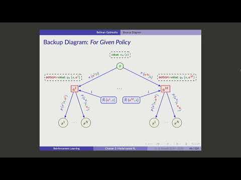
5:00 Backup Diagrams: Tracing State, Action, and Transition Nodes

A backup diagram alternates state-value nodes, action-value nodes, and next-state nodes.
Policy probabilities connect states to actions, while environment transition probabilities connect actions to successor states.
The tree represents forward time, even when a transition returns to the same state, as when a grid-world move hits a wall.

10:00 Policy Branching and Immediate Rewards in Bellman Backups

A deterministic policy assigns probability 1 to one action and 0 to the alternatives; a stochastic policy can branch across actions.
Each action produces an expected immediate reward and a distribution over next states.
Chess illustrates how branching across actions and states can make a full search tree grow exponentially.

15:00 Computing Action Values from Successor-State Values

Qπ(s,a) equals the expected immediate reward plus the probability-weighted value of successor states.
The backup averages each possible next-state value using the transition probabilities after action a.
For a finite MDP, writing one Bellman equation per state-action pair yields a system of equations for the action values.

20:00 State Values as Policy-Weighted Action Values

Vπ(s) is the policy-weighted average of the action values available in state s.
Combining policy and environment transitions gives a policy-dependent state transition distribution.
The compact Bellman equation expresses state value as expected immediate reward plus expected next-state value.

25:00 From Policy Evaluation to Bellman Optimality

Bellman equations evaluate a specified policy, but finding the best policy requires maximizing value at each state.
For a fixed state, Vπ(s) is an average of the available action values and cannot exceed their maximum.
Choosing an action with maximum action value achieves that upper bound.

30:00 Greedy Actions and the Optimal Policy

An optimal policy selects an action with the greatest optimal action value in each state.
The relevant Q-value includes future rewards under subsequent optimal behavior, not just the immediate reward.
This gives the policy-improvement rule: replace an action when another action has a higher evaluated Q-value.

35:00 The Mutual Dependence of Optimal Policies and Values

The optimal policy is greedy with respect to Q*, while Q* itself reflects behavior under the optimal policy.
This apparent circularity becomes useful as a recursive characterization rather than a direct one-step calculation.
A claimed optimal policy can be checked by evaluating its action values and verifying that its choices maximize them.

40:00 Deriving the Bellman Optimality Equation

Substitute the optimal value of each successor state into the action-value Bellman equation.
Taking the maximum over actions gives V*(s) = maxₐ E[r + V*(s′)] when the discount factor is 1 in the examples.
The resulting equations couple the optimal values of all states and include a maximum, making them nonlinear.

45:00 Four-Cell Grid World: Rewards and Terminal State

In the four-cell example, state 0 is terminal and has value 0.
Actions that move into a new cell earn −1, while actions that hit a wall earn −0.5.
With discount factor 1, each candidate action value combines its immediate reward with the value of the resulting state.

50:00 Writing Optimal-Value Equations for the Grid World

For state 1, moving left reaches terminal state 0, moving down reaches state 3, and wall collisions return to state 1.
The Bellman optimality equation takes the maximum over these reward-plus-successor-value expressions.
Equations for states 1, 2, and 3 form a coupled system because each state can depend on the others.

55:00 Solving the Grid World and Recovering the Optimal Policy

The maximum terms make direct algebra less straightforward than solving a linear policy-evaluation system.
For the four-cell grid, the optimal values are 0 at the terminal state, −1 at states 1 and 2, and −2 at state 3.
Once V* is known, compute each Q*(s,a) with the standard Bellman equation and select a maximizing action.

1:00:00 Why a Deterministic Optimal Policy Always Exists

For a finite MDP, at least one deterministic optimal policy exists by choosing a maximizing action in each state.
If multiple actions tie for the maximum Q-value, any of them is optimal.
A policy can randomize among tied maximizing actions without reducing expected value.

1:05:00 Tied Optimal Actions in the Four-Cell Grid

At state 3, moving left and moving up both produce the same optimal action value, −2.
Choosing either action deterministically is optimal, and randomizing between them is also valid.
The action-value comparison is based on expected returns, so it does not require deterministic rewards.

1:10:00 Dynamic Programming as Fixed-Point Iteration

The Bellman equations define fixed points: applying the corresponding update should leave the correct value function unchanged.
Dynamic programming can solve such equations by repeatedly updating an initial value estimate.
Policy evaluation iterates the Bellman equation for a fixed policy; value iteration iterates the Bellman optimality equation.

1:15:00 How Recursive Updates Approach a Fixed Point

For a scalar equation x = f(x), fixed-point iteration uses xₖ₊₁ = f(xₖ) until successive estimates are sufficiently close.
The equation x = −1/(2+x) has solution −1, and iteration from 0 approaches that solution.
Convergence depends on the update function and starting point; an equivalent rearrangement can diverge from some initial values.

1:20:00 Choosing Between Policy Evaluation and Value Iteration

A fixed policy produces Bellman equations that can be solved iteratively to obtain Vπ.
Policy iteration combines that evaluation with a separate policy-improvement step.
Value iteration instead applies recursive updates directly to the Bellman optimality equation, then recovers a policy from the resulting values.

1:25:00 Policy Evaluation: Initialize Values for Every State

For n states, a value function can be stored as a vector or table of n numbers.
Start with an initial estimate, commonly zero for every state, while ensuring terminal-state values are set to zero.
The transition model, reward expectations, and policy are treated as known in this model-based procedure.

1:30:00 Policy Evaluation Updates from Expected Rewards and Transitions

For each state, calculate the expected immediate reward using the policy and reward distribution.
Calculate expected next-state value by weighting each successor’s current estimate by its policy-dependent transition probability.
Replace the estimate with the Bellman right-hand side and repeat across states.

1:35:00 Stopping Policy Evaluation with a Convergence Tolerance

One sweep of Bellman updates produces a new value vector from the previous vector.
Track the largest absolute change across states and stop when it falls below a threshold ε.
A smaller ε gives a more accurate estimate; initializing terminal states to zero prevents ambiguous fixed points in unusual cases.

1:40:00 Evaluating a Fixed Grid-World Policy

Under the example policy, states 1 and 2 transition to state 0, while state 3 transitions to state 2.
Nonterminal moves receive immediate reward −1, and the terminal state has value 0.
Starting from zero, one update sets states 1 and 2 to −1; the next propagates the value to state 3 as −2.

1:45:00 Policy Improvement: Replace Actions with Higher Q-Values

After evaluating π, calculate Qπ(s,a) for every available action in each state.
If π does not choose an action with maximum Qπ, change its choice to a maximizing action.
The policy-improvement result is at least as good as the previous policy, though it may still be suboptimal.

1:50:00 Why Greedy Policy Improvement Increases Value

Improvement compares each candidate first action using Qπ, which accounts for following the old policy afterward.
Although the improved policy changes future behavior, the policy-improvement theorem guarantees its value is no worse.
Repeating evaluation and improvement can continue until no state has a better action.

1:55:00 Grid-World Policy Improvement from a Poor Initial Choice

A policy that moves down from state 1 earns a return of −3 by taking a longer route to the terminal state.
Changing state 1 to move left gives Qπ(1,left) = −1 because it reaches the terminal state immediately.
The other states already choose maximizing actions in this example, so the improvement changes only state 1.

2:00:00 Policy Iteration Alternates Evaluation and Improvement

Policy iteration starts with an initial policy, evaluates it, computes action values, and improves its choices.
The improved policy is evaluated again, and the cycle repeats until the policy no longer changes.
Evaluation and improvement form nested processes: value updates occur inside each policy-improvement round.

2:05:00 Warm-Starting Policy Evaluation Speeds Later Rounds

After improving a policy, initialize evaluation with the previous policy’s value vector rather than starting from zero.
Because policy improvement often changes only a few actions, the prior vector may already be close to the new policy’s values.
This warm start can reduce the number of Bellman sweeps needed in later policy-iteration rounds.

2:10:00 Value Iteration Skips Full Policy Evaluation

Value iteration updates values using the maximum action value rather than averaging over a fixed policy.
It does not wait for a policy evaluation to converge before taking another greedy update.
Once the values converge, compute Q* and select maximizing actions to obtain the optimal policy.

2:15:00 The Value-Iteration Bellman Update

Initialize V₀, often as zeros, and update every state with the maximum expected reward-plus-successor-value over available actions.
Repeat the update until the maximum state-value change falls below a convergence threshold.
Unlike policy evaluation, this update has no fixed policy π; the maximum operator supplies the greedy choice.

2:20:00 Policy Evaluation and Value Iteration Share Action Calculations

Both algorithms calculate reward-plus-next-value terms for each state-action pair.
Policy evaluation averages those terms according to π, whereas value iteration takes their maximum.
Value iteration can be understood as continually applying a greedy improvement without fully evaluating intermediate policies.

2:25:00 Sixteen-State Grid World: Random-Policy Evaluation

The textbook-style 4×4 grid has 16 cells, terminal states 0 and 15, and a reward of −1 for every move.
From each nonterminal cell, the initial policy chooses up, down, left, or right with probability 1/4.
Starting with zero values, the first Bellman sweep assigns −1 to nonterminal states because every move costs −1 and successor estimates are zero.

2:30:00 Improving the 4×4 Grid Policy Toward Terminal States

Repeated evaluation of the random policy propagates increasingly accurate values across the 4×4 grid.
At a cell next to a terminal, moving into that terminal gives action value −1 and is better than continuing to wander randomly.
Greedy improvement first fixes actions near terminals, then the improved behavior propagates into more distant cells.

2:36:00 Convergence, Approximation, and Generalized Policy Iteration

Exact policy iteration can require multiple evaluations, while value iteration may need many updates because it solves the nonlinear optimality equation directly.
In practice, policy evaluation is often stopped after a fixed number of sweeps; improving the policy from approximate values yields generalized policy iteration.
One evaluation sweep per improvement approaches value iteration, while more evaluation sweeps approach full policy iteration; both converge to the same optimum when carried to convergence.

Summary, takeaways, and chapters were generated by AI from the video's transcript and may contain errors. The video belongs to its creator, Ali Bereyhi.