RL @ ECE-UofT - Lecture 01: RL Framework
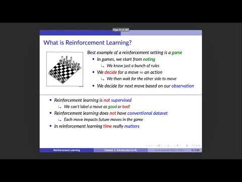 Watch on YouTube →
Overview
Ali Bereyhi introduces reinforcement learning as learning how an agent should act by interacting with an environment, then formalizes the framework through actions, rewards, observations, states, transitions, and discounted return. A two-company multi-armed bandit example shows how sampling trades off exploration and reward, while chess, tic-tac-toe, pendulum control, trading, and FrozenLake illustrate stochastic environments and Markov modeling.
Key takeaways
- Reinforcement learning is an online decision process: actions affect which observations and rewards become available, unlike training from a fixed labeled dataset.
- In the two-company bandit, choosing the higher-mean company A yields $600 per day versus B’s $400, but the learner must discover that difference from noisy samples.
- A one-day payment comparison selects A with probability about 0.818 under the example’s Gaussian assumptions; increasing the number of samples improves reliability at the cost of exploration time.
- The Markov model assumes the current state contains the relevant information for predicting the next state and reward after an action; missing information is represented as stochasticity.
- The discount factor γ controls how strongly the agent values future rewards: γ = 0 focuses on immediate outcomes, while values near one encourage longer-horizon planning.
- FrozenLake makes the RL model concrete: grid position is the state, four directions are actions, holes and the goal define rewards, and slippery movement introduces stochastic transitions.
Chapters
0:00
Reinforcement Learning as Learning to Interact with an Environment
- Ali Bereyhi frames reinforcement learning as an agent—such as an algorithm, machine, or computer—learning how to interact with an environment.
- The environment imposes rules the agent cannot control; an action changes the environment and produces feedback.
- A person moving a leg illustrates the loop: act, observe a changed position or painful collision, and adjust future behavior.
4:00
Why Reinforcement Learning Is Not Conventional Supervised Learning
- Supervised learning uses labeled examples, while unsupervised learning finds patterns without labels; reinforcement learning learns from environment interactions.
- A chess move has no context-free good-or-bad label because its value depends on the opponent and the evolving position.
- Rewards may arrive only at the end of a task, such as a chess win or loss, rather than with every observation.
7:00
Chess, AlphaZero, and Online Decision-Making
- Chess illustrates online learning: each move affects later positions, and the agent gathers information while playing rather than from a fixed dataset.
- Ali Bereyhi cites AlphaZero, developed by David Silver’s DeepMind team, as a system that learned board games through self-play and neural-network methods.
- An early mistake may have consequences several moves later, so evaluating actions requires reasoning about future outcomes.
13:00
The Multi-Armed Bandit as a Simple Reinforcement-Learning Problem
- Bereyhi introduces the multi-armed bandit, a classic statistical decision problem associated with work dating to 1952.
- The example turns each bandit arm into a company renting a programming robot, making each choice an action with a random payment.
- The simplified setup establishes notation and intuition before moving to more complex reinforcement-learning environments.
15:30
Two Companies with Different Payment Distributions
- Company A pays a Gaussian-distributed daily amount with mean $600 and standard deviation $100.
- Company B pays a Gaussian-distributed daily amount with mean $400 and standard deviation $200.
- The policy, written as πₜ, selects which company receives the robot on day t; the payment Rₜ is random even after the choice.
18:10
Expected Return Defines the Bandit’s Optimal Policy
- The example adopts average expected payment as its objective, rather than preferring a riskier option that sometimes pays more.
- Since A’s mean is $600 and B’s is $400, the optimal policy—if the distributions are known—is to choose A every day.
- The long-run average motivates the law of large numbers, but the practical learner does not know the payment distributions in advance.
22:00
Unknown Company Behavior Makes Learning Necessary
- In practice, the agent cannot simply choose A from the given means because those statistics are not available to it.
- It must infer company behavior from observed payments and use those samples to choose future actions.
- The performance question becomes how much reward the learned policy loses compared with the optimal $600-per-day benchmark.
26:30
Random Choice Establishes a $500-per-Day Baseline
- A coin-flip policy chooses A or B with equal probability and therefore earns an expected (600 + 400) / 2 = $500 per day.
- Against the $600 optimal expected payment, random selection incurs $100 of average regret per day.
- Regret measures the gap between the optimal return and the return generated by a policy.
28:30
One-Day Sampling and the Winner-Stays Policy
- The learner samples A on day one and B on day two, then compares the two observed payments.
- For all subsequent days, it keeps choosing whichever company paid more during the initial test.
- This policy uses observed outcomes rather than known company means, but a single noisy sample can lead to a lasting bad choice.
34:30
Computing the One-Day Policy’s Selection Probability
- Let Δ = R₁ − R₂; the policy selects A precisely when Δ is positive.
- For independent Gaussian payments, Δ is Gaussian with mean $200 and variance 100² + 200², giving a standard deviation of about $223.6.
- The probability that the one-day comparison selects A is approximately 0.818, or about 81%.
40:00
One-Day Testing Improves Expected Return but Is Unreliable
- The initial comparison is more rewarding on average than random choice because the learner uses payment evidence to select a company.
- However, the approximately 19% chance of selecting B means some learners remain with the lower-paying company indefinitely.
- Expected return alone does not describe the policy’s risk; Bereyhi identifies variance as another useful measure of reliability.
45:30
More Samples Reduce the Risk of Choosing the Wrong Company
- Instead of sampling each company for one day, the learner can spend D days with A and D days with B.
- It compares the cumulative payments S_A and S_B, then keeps working with the company whose total was larger.
- Using multiple observations makes the decision less sensitive to an unusually high or low payment on a single day.
51:30
Cumulative Payment Differences Become More Informative
- For D samples per company, Δ = S_A − S_B is Gaussian under the example’s independent Gaussian assumptions.
- Its mean is D(μ_A − μ_B), so with the stated companies it grows as 200D.
- The standard deviation grows more slowly than the mean, making the probability of correctly identifying A increase as D increases.
58:00
Exploration Cost, Regret, and the Limits of the Bandit Model
- The probability of selecting A is computed from a Gaussian tail probability; as D grows, that probability approaches one.
- For sufficiently large D, Bereyhi gives an approximate regret of 200D/T, highlighting that testing has a cost proportional to its share of the total horizon.
- Sampling first can reduce long-run regret when T is much larger than D, but spending too much of a short horizon testing leaves fewer days to exploit the better company.
- The calculation assumes an idealized independent payment model; real environments may violate it, so models must be tested and revised against practical behavior.
1:04:00
The Core Reinforcement-Learning Components and Notation
- The framework has an agent, an environment, and their interaction; the company-rental example supplies a concrete instance of each.
- The agent chooses an action Aₜ from possible actions a₁ through aₘ, and receives a reward Rₜ₊₁ after acting.
- Bereyhi also introduces the observation Yₜ₊₁, which can provide information beyond the reward, such as an opponent’s chess move.
- The action, reward, and observation are modeled as random variables in the general stochastic framework.
1:10:00
Interaction Trajectories and the Agent’s Information
- After action Aₜ, the agent receives reward Rₜ₊₁ and observation Yₜ₊₁; that feedback informs the next action.
- A trajectory can be represented as a sequence of actions followed by their resulting rewards and observations.
- In chess, an opponent’s move can be an observation even when it does not immediately produce a win-or-loss reward.
1:17:00
Future Return and the Discount Factor γ
- The future return from time t sums rewards beginning with Rₜ₊₁, rather than rewards already received.
- A discount factor γ between zero and one weights later rewards by γⁱ, limiting infinite-horizon sums and expressing reduced emphasis on distant outcomes.
- With γ = 0, the agent is short-sighted and optimizes immediate reward; with γ near one, it accounts more strongly for the future.
- Bereyhi notes that γ is a design choice and is often set to one when the return remains mathematically well-defined.
1:23:30
Stochastic Environments and Countable State Spaces
- The course adopts a stochastic, state-dependent framework that can represent uncertain outcomes across many applications.
- An environment is modeled as having a finite or countable set of states, although the number of possibilities can be enormous.
- A bit string of length n alone has 2ⁿ possible configurations, illustrating why practical state spaces can grow rapidly.
- Continuous systems, such as a robot arm’s angles, can initially be approximated by discretizing or quantizing their values.
1:29:00
True State Versus Partial Sensor Information
- A robot’s full environment state may include joint angles, surface friction, wind, lighting, and other physical conditions.
- Sensors usually reveal only part of that state; Bereyhi presents full-state access as an idealization and suggests treating unobserved factors as additional randomness.
- More advanced partial-observation frameworks exist, but the course initially uses a fully observed state model for tractability.
1:36:00
Markov Property, Reward Function, and Transition Function
- The Markov assumption says the next state depends on the current state and action, not on the full history when the relevant information is captured in the state.
- The reward mapping takes a state and action and returns a possible reward; the transition mapping determines the next state.
- Both mappings may be stochastic: the same state-action pair can lead to different rewards or successor states.
- The state should contain useful information about the environment; factors omitted from it are absorbed into the stochastic model.
1:42:30
Tic-Tac-Toe: Encoding Board States and Opponent Moves
- The agent is one tic-tac-toe player; the environment includes the board and the opponent’s behavior.
- Bereyhi encodes a 3×3 board using cells numbered 0 through 8 and represents a state by the played cells and their marks.
- After the agent chooses cell 6, the next state also depends on the opponent’s subsequent move, making the transition stochastic.
- A simple reward scheme assigns +1 for a win, −1 for a loss, and 0 when play continues; opponent behavior determines transition probabilities.
1:50:00
Pendulum Control and Trading as Stochastic RL Tasks
- In a pendulum-style control task, actions push left or right; rewards can be positive while the pole remains upright and zero after it falls.
- A realistic physical transition can depend on friction, wind, and other conditions, while a simplified model treats unobserved variables as random.
- A trading agent might choose to buy or sell, with the environment including market conditions, portfolio, transaction rules, and news.
- Trading illustrates partial state information: many influences on prices are inaccessible, so the transition model is uncertain.
1:56:10
FrozenLake: States, Actions, Rewards, and Slippery Transitions
- FrozenLake represents the state as the current grid-cell index and offers four actions: left, down, right, and up.
- The goal is to reach the prize; falling into a hole ends the task, and movement can slip away from the intended direction with probability P.
- The reward scheme can assign +1 at the destination, −1 at a hole, and 0 elsewhere; setting P to zero makes movement deterministic.
- At a cell beside a hole, an intended move may have a safe outcome with probability 1−P and a harmful sideways outcome with probability P.
2:00:00
Gymnasium FrozenLake Setup and Assignment Preview
- Bereyhi introduces Gymnasium as a library of prebuilt environments, including FrozenLake for practical reinforcement-learning experiments.
- A sample setup selects a 4×4 FrozenLake environment, configures the slippery option, and enables human rendering.
- The agent can sample or choose actions, apply them to the environment, and inspect the resulting state and reward.
- FrozenLake is slated for Assignment 1; the lecture closes by noting that tutorials begin later.
Summary, takeaways, and chapters were generated by AI from the video's transcript and may contain errors. The video belongs to its creator, Ali Bereyhi.