RL @ ECE-UofT - Lecture 04: Generalized Policy Iteration via Monte-Carlo and Temporal Difference
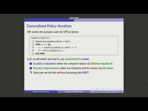 Watch on YouTube →
Overview
Ali Bereyhi develops generalized policy iteration for model-free reinforcement learning by replacing Bellman-equation evaluation with sampled returns, first through Monte Carlo and then through one-step temporal-difference learning. The lecture derives incremental value and action-value updates, compares Monte Carlo’s unbiased but higher-variance estimates with TD’s lower-variance bootstrapped targets, and shows how greedy policy improvement turns either evaluation method into an approximate control loop.
Key takeaways
- Monte Carlo policy evaluation estimates Vπ(s) by averaging complete discounted returns; with infinitely many visits to every state, the law of large numbers gives convergence to the true value.
- The incremental update V̂ ← V̂ + α(G − V̂) supports online averaging, with α = 1/K recovering the arithmetic mean and constant α producing geometric weighting.
- TD0 replaces the complete return G with the one-step target R_{t+1} + γV̂(S_{t+1}), allowing updates after each transition without waiting for an episode to terminate.
- Monte Carlo targets avoid bootstrapping and can be unbiased under suitable sampling, while TD targets often have lower variance and learn faster but can inherit bias from imperfect next-state estimates.
- Action-value estimates enable generalized policy iteration without a known transition model: evaluate Qπ(s,a) from sampled data, then choose the highest-valued action at each state.
- TDn and TD lambda interpolate between TD0’s one-step bootstrap and Monte Carlo’s full return, trading off how much observed trajectory information is used before bootstrapping.
Chapters
- Reviews value functions, action-value functions, Bellman equations, policy iteration, and value iteration.
- Model-free RL assumes an MDP exists but does not provide its transition probabilities.
- The goal is to retain policy evaluation and improvement without explicitly solving the environment model.
- Generalized policy iteration alternates policy evaluation and policy improvement, potentially using only partial evaluation before improving.
- One evaluation update per improvement approaches value iteration; thorough evaluation approaches policy iteration.
- Monte Carlo estimates expectations from sampled outcomes when the distribution is unknown.
- Repeated measurements of a random variable can estimate its expectation by averaging independent samples.
- The sample mean is itself random; the central limit theorem describes its error as approximately Gaussian with variance shrinking as sample count grows.
- For RL, each sampled episode supplies a return that acts as one sample of a state’s value.
- Start from state s, follow a fixed policy until termination, and sum discounted rewards to obtain one return sample.
- Repeating the episode from the same starting state provides multiple samples whose average estimates Vπ(s).
- Monte Carlo samples trajectories instead of enumerating every branch of the unknown transition tree.
- Initialize an estimate for the target state, sample K episodes under the fixed policy, and compute each episode’s discounted return.
- The batch estimate is the sum of K returns divided by K.
- The basic algorithm can estimate one selected state at a time, which motivates more efficient updates.
- After K samples, rewrite the average using the previous estimate and the new return.
- The online update is estimate ← previous estimate + (1/K) × (new sample − previous estimate).
- With a fixed step size α, the update becomes a weighted moving average rather than uniform averaging.
- A step size of 1/K reproduces the arithmetic mean as samples accumulate.
- A constant α gives newer samples persistent influence through geometric weighting.
- The lecture recommends treating α as a tunable hyperparameter because too-small or too-large updates can worsen estimates.
- A single trajectory visits multiple states, so its suffix returns can provide samples for every visited state.
- For state S1, the relevant return begins with the reward after S1, not with rewards received before reaching it.
- Time-indexed states can refer to the same physical state, such as repeatedly hitting a wall in a grid.
- Initialize a value table for all states, then begin episodes from varied starting states and follow the evaluation policy.
- Each occurrence of a visited state supplies a return sample and can update that state’s estimate.
- A state may appear multiple times in one trajectory, producing multiple updates under every-visit sampling.
- Compute returns efficiently by starting at the end with G = 0 and moving backward through rewards.
- At each earlier step, update the return as G ← reward + γG.
- Once a state’s return is computed, use it in the incremental value update; this avoids separately summing each trajectory suffix.
- Monte Carlo evaluation requires complete episodes before updating the visited states’ returns.
- If every state is visited infinitely often, the law of large numbers implies convergence to the true policy value.
- In large environments, rare states may require impractically many episodes to observe often enough.
- A randomly acting grid-world policy illustrates values such as 0 for a terminal state, about −4.5 for neighboring cells, and −6 for a corner.
- Monte Carlo estimates fluctuate early but approach known values as episode counts rise.
- Root mean squared error can compare estimates with exact values in a small environment; step size α affects the error non-monotonically.
- Policy improvement needs action values, so Monte Carlo can estimate Qπ(s,a) from returns after taking action a in state s.
- Store estimates in a state-by-action Q table, initialized to zero.
- Each visited state-action pair receives a return sample from the trajectory that follows it.
- For each state, select the action with the largest estimated Q value.
- A deterministic greedy policy assigns probability 1 to the maximizing action and 0 to the others.
- Monte Carlo generalized policy iteration alternates sampled Q evaluation with greedy policy improvement.
- An ideal evaluation of a new policy could restart its value table from zero, but this costs additional computation.
- Carrying forward the previous Q table can provide a useful warm start as successive policies become more similar.
- Warm starts can reduce variance and computation, but old estimates may introduce bias when the new policy differs substantially.
- Monte Carlo GPI assumes time to collect episodes for policy evaluation before changing the policy.
- The greedy update uses limited sampled evidence, so it may make large, variable changes early in training.
- With sufficient samples at each iteration, the method is expected to approach optimal values and a better policy, though practical runs usually remain approximate.
- Complete-return Monte Carlo naturally fits episodic tasks whose trajectories reach terminal states.
- For continuing tasks, truncate a trajectory after a large horizon T; when γ < 1, distant rewards have diminishing influence.
- A window of W steps can be left beyond the last state updated, reducing the error caused by truncating too close to the endpoint.
- The Bellman equation writes a state value as immediate reward plus γ times the expected value of the next state.
- If a next-state value estimate were available, one transition could provide a value target without waiting for episode termination.
- This bootstrapped target replaces the full Monte Carlo return with reward plus an estimate of future value.
- For a transition from S0 to S1 with reward R1, the one-step target is R1 + γV̂(S1).
- Averaging such targets estimates the Bellman expectation; an incremental update can apply each transition immediately.
- TD evaluation does not require a terminal state after every update, making it suitable for continuing environments.
- TD0 can begin with every state value set to zero and update V̂(S_t) from the observed reward and current estimate of V̂(S_{t+1}).
- As transitions are observed, updated next-state estimates feed into later updates for preceding states.
- Bootstrapping propagates information through the value table, but early targets inherit error from initially poor estimates.
- For each transition, TD updates the current state using R_{t+1} + γV̂(S_{t+1}), even if the trajectory ends at an arbitrary time limit.
- The estimate for a state can be updated as soon as its next state and reward are observed.
- This differs from Monte Carlo, which must wait for the episode’s complete return before updating.
- The action-value Bellman target is the immediate reward plus γ times the value of the next state, conditioned on the current state and action.
- A Q table can produce V̂(s) by averaging action values according to the evaluation policy’s action probabilities.
- TD evaluation of Q values can be followed by the same greedy improvement used in Monte Carlo GPI.
- The toy environment has green, blue, and red light states, one button-press action, and red as a terminal state.
- Each press yields reward 0 or 1; green and blue allow play to continue.
- Six example trajectories supply different amounts of evidence for estimating the values of green and blue.
- Monte Carlo treats each suffix beginning at a blue state as a sample and sums rewards until red.
- With the lecture’s example of eight blue-state return samples, four returns of 1 and four of 0 give an estimated blue value of 0.5.
- Green appears only once in the example and its observed complete return is 0, illustrating the unreliability of sparse coverage.
- TD first updates blue from observed transitions; the example’s blue estimate reaches about 0.5.
- When a green transition yields reward 0 and leads to blue, TD uses 0 + V̂(blue), producing a green estimate of about 0.5.
- Monte Carlo instead uses green’s single observed complete return of 0, while TD reuses learned information about what follows blue.
- Monte Carlo estimates complete returns without relying on intermediate-state value estimates.
- TD uses the MDP’s recursive structure and observed transitions to reuse next-state estimates.
- The lecture notes a transcription or slide-count error in the button-game sample totals, so the numerical counts are illustrative rather than definitive.
- TD can learn efficiently when the environment is well represented as an MDP with meaningful states and transitions.
- In settings such as asset trading, the current price alone may omit important causes of future changes, making the assumed state representation inadequate.
- Monte Carlo avoids bootstrapping from intermediate estimates, while TD can exploit structure when its state model is appropriate.
- The order in which trajectories are processed can affect intermediate TD estimates because later updates use the current table.
- One practical approach is to sample a batch of trajectories and pass over the same batch multiple times.
- After repeated updates on that batch, collect new trajectories and continue evaluating the policy.
- In the random-walk comparison, TD0 error falls faster than Monte Carlo error for the illustrated step-size settings.
- Monte Carlo averages complete returns and is unbiased under appropriate independent sampling, but can have higher variance.
- TD often has lower variance and learns faster, but its bootstrapped estimates may retain bias and reach an error floor.
- Bias is the gap between an estimator’s long-run average and the true value; variance measures its fluctuations around that average.
- TD targets inherit error from current next-state estimates, while Monte Carlo targets use sampled returns through termination.
- The useful tradeoff depends on sample availability, state-space size, step size α, and how faithfully the task fits an MDP.
- TD-based policy iteration evaluates action values with TD updates, then improves the policy greedily.
- TD0 bootstraps after one transition; TDn uses n observed rewards before bootstrapping from a later state value.
- TD lambda combines return estimates across multiple horizons, bridging one-step TD and full Monte Carlo; the lecture previews it before moving toward online control.
Transcript excerpt
0:03 Okay, model free reinforcement learning. So, uh we already talked about the model base, right? Uh so just a quick recap. Uh what we have done up to this point, we basically talked about the reinforcement learning story. So you have an agent, you have the environment. The agent is trying to somehow interact with this environment. side going to maximize the kind of return it gets from the environment. Right? So that is the whole story. We talked last time about the modelbased reinforcement learning. What is the idea there? You do know the environment. Right? You can describe the environment using one MDP a mark of decision process. Right? Now this MDP when you when you have it what can you do? You
0:53 can define first of all parameter which is somehow evaluating your policy. What was that function that evaluates your policy that is what do you use to evaluate your policy? What does say your policy is good or bad? There is something we define for that policy. >> Value function. Right? So we talked about the value function. The value function it's evaluating your policy. Right? And then there is one other thing we called it action value. So it was it basically the same thing but you also take into account the first action that you do. Now once we have this one we can define the notion of optimal policy and then if you have the MDP the story was not very complicated
1:42 right because we could develop the recursive equation the Bellman equation. The Bellman equation is telling you how you can write down the value of one particular state in terms of the future state, right? And then you can use this recursive property plus the fact that you know what are the chances of going
This is the start of the transcript. Save this video free for the whole transcript, searchable and time-coded.
Related notes
Summary, takeaways, and chapters were generated by AI from the video's transcript and may contain errors. The video belongs to its creator, Ali Bereyhi.