RL @ ECE-UofT - Lecture 02: MDPs and Bellman

Overview

Ali Bereyhi defines policies, state-value and action-value functions, and policy optimality, then models finite environments as Markov decision processes (MDPs). He derives the Bellman equations as recursive ways to evaluate a fixed policy and its actions, setting up value iteration and policy iteration for finding optimal behavior.

Key takeaways

A policy π(a|s) is a distribution over actions for every state; deterministic behavior is the special case where one action has probability 1.
Vπ(s) evaluates expected long-term return from a state, while Qπ(s,a) evaluates return after a specified first action and policy-controlled behavior afterward.
An MDP’s joint distribution p(r,s′|s,a) determines both reward and transition models through marginalization, and the Markov property removes dependence on earlier history.
The Bellman equation replaces an expansion over an entire trajectory with immediate reward plus discounted expected value of the next state.
For a known finite MDP and fixed policy, policy evaluation produces n equations for n state values; action-value evaluation produces n×m equations.
Optimal policies maximize long-term action value, and Bellman-based value iteration or policy iteration can improve policies toward optimality.

Chapters

0:00 Reinforcement Learning: Agent, Environment, Actions, and Rewards

An agent interacts with an environment by observing its state and choosing an action.
The environment changes state and returns a reward after an action.
The agent’s objective is to learn behavior that collects as much reward as possible.

1:36 Policies as State-Conditioned Action Distributions

A policy π(a|s) assigns a probability to each action available in state s.
For a finite set of m actions, the probabilities across the actions form a distribution.
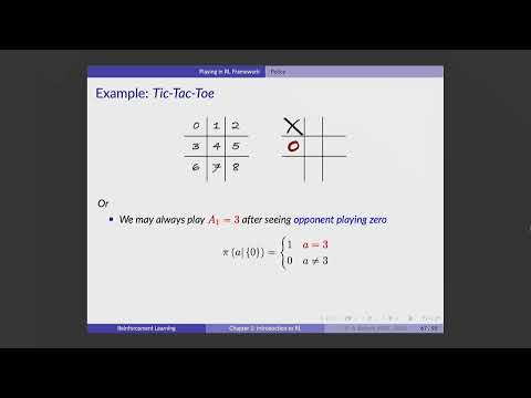
A deterministic choice is represented by a one-hot distribution, such as probability 1 for one action and 0 for all others.

5:48 Tic-Tac-Toe: Policies Respect Legal Moves

In tic-tac-toe, the board configuration is the state and each available cell is a possible action.
If the opponent has already occupied cell 0, the policy must assign action 0 probability 0.
A stochastic policy could select among cells 1, 3, and 4 with probability 1/3 each.

12:06 A Policy Is a Table Covering Every State

A policy specifies an action distribution separately for each possible state, rather than only for the current turn.
With n states and m actions, the policy can be viewed as an n-by-m table of probabilities.
In tic-tac-toe, the distribution changes as the board changes, while the policy rule covers all possible board states.

14:41 State Value Measures Expected Future Return

The value function Vπ(s) is the expected future return when starting in state s and following policy π.
Return includes rewards collected over the subsequent trajectory, so it evaluates long-term consequences rather than one move.
The policy appears in the value notation because different action choices can produce different future rewards.

18:21 Discounted Return and Random Trajectories

The return from time t is the sum of future rewards, typically discounted by powers of γ.
Policy choices, state transitions, and rewards can all be stochastic, producing different trajectories on repeated runs.
The value is the expectation of that return conditioned on starting in state s.

21:20 Computing Expected Rewards from Policy and Environment

To compute the immediate reward expectation, average the reward distribution for each action in state s.
Weight each action’s expected reward by its policy probability π(a|s), then sum across actions.
Later rewards require accounting for the transition to a next state, the next policy action, and the corresponding reward distribution.

34:33 Tic-Tac-Toe Opponent and Policy Rules

Bereyhi defines a simple opponent that takes available corners, blocks an immediate threat, and wins when it can complete a line.
The agent’s first policy imitates these tactical rules but starts by playing the next available cell.
The opponent is treated as part of the environment, allowing its behavior to be modeled as a transition rule.

40:27 Comparing Tic-Tac-Toe Policies by Their Outcomes

Under the next-cell policy, the modeled opponent and agent follow a deterministic trajectory ending in a draw.
A second policy that starts in a corner can reach a position where either random defensive move still allows the opponent to win.
The state value for that losing position is −1, illustrating that a policy’s value summarizes expected outcomes.

45:13 Action Value Qπ(s,a): Evaluating a Chosen Move

The action-value function Qπ(s,a) is expected return after taking action a in state s and following π afterward.
The immediate reward depends on the state and specified action, not on the policy.
The policy affects future rewards after the initial action changes the state.

49:30 A Mixed Tic-Tac-Toe Policy Produces Value −0.5

The mixed policy selects the next-cell strategy 50% of the time and the corner strategy 50% of the time.
From the initial state, the first action values are 0 for the draw-producing move and −1 for the losing move.
Averaging these outcomes under the policy gives state value −0.5.

54:49 Policy Ordering and the Definition of Optimality

Policy π1 is better than π2 when Vπ1(s) is at least Vπ2(s) for every state.
An optimal policy π* is at least as valuable as every alternative policy across all states.
An optimal policy need not be unique; different actions can have equal long-term value.

1:04:01 Model-Based and Model-Free Reinforcement Learning

Model-based methods use known transition and reward distributions to calculate values and improve a policy.
Model-free methods estimate values from repeated interaction, such as averaging wins, losses, and draws over many games.
The distinction is whether the algorithm relies on an explicit environment model.

1:09:01 Large State Spaces and Deep Reinforcement Learning

Chess has an enormous state space; the lecture contrasts estimates around 10^40–10^43 positions with Shannon’s much larger 10^120 figure.
When explicit value tables are impractical, a neural network can approximate values from sampled states.
Deep reinforcement learning can combine neural approximators with either model-based or model-free approaches.

1:13:37 Terminal States and Episodic Tasks

A terminal state transitions to itself for every action and returns reward 0 thereafter.
Its value is 0 under any policy because no further reward is collected.
An episode is a trajectory from an initial state to a terminal state; episode lengths can vary.

1:17:35 Frozen Lake Policies and Multiple Optimal Routes

In Frozen Lake, falling into a dashed hazard cell ends the episode, making that cell terminal.
A policy can be deterministic or stochastic; at cell 9, for example, it may choose right or down with probability 1/2 each.
When there is no slipping, multiple routes to the goal can all be optimal if each achieves the maximum reward.

1:24:32 Model-Based Reinforcement Learning and the MDP Setup

An MDP provides a mathematical model of the environment, which may come from physical laws or an explicit behavioral model.
The lecture assumes a finite set of states, actions, and rewards, even if these sets are large.
The goal remains finding an optimal policy, with this section focusing on environments whose model is known.

1:27:02 The Markov Property and Stationary Dynamics

An MDP models the joint distribution of next reward and next state given the current state and action.
The Markov property means the next outcome depends on the current state and action, not the full earlier history.
The transition and reward dynamics are assumed stationary, meaning their distributions do not change over time.

1:31:45 Marginalizing the MDP into Reward and Transition Models

The joint model p(r,s′|s,a) contains the environment’s reward and transition information.
Summing over next states gives the reward distribution p(r|s,a).
Summing over rewards gives the transition distribution p(s′|s,a).

1:34:30 Gridworld: Reward Shaping for the Shortest Path

The four-cell gridworld uses the upper-left cell as its destination and treats it as terminal.
Each move receives reward −1 to favor reaching the goal quickly; hitting a wall receives −0.5 in this example.
The reward values encode the shortest-path objective without requiring a separate distance calculation.

1:37:23 Writing Gridworld Transitions and Terminal Behavior

From cell 3, moving up deterministically reaches cell 1 and returns reward −1.
From terminal cell 0, every action leaves the agent in cell 0 and returns reward 0.
Transition diagrams can show reachable states, action labels, and rewards; wall collisions create self-loops.

1:43:16 Immediate Reward Depends on the Policy’s Action Choices

The reward for a specified state-action pair comes directly from the MDP and does not itself depend on the policy.
At a boundary cell, moving into the grid may yield −1 while hitting the wall yields −0.5.
With four actions chosen uniformly, two moves at the example cell yield −1 and two yield −0.5, for expected immediate reward −0.75.

1:47:14 Why Immediate Reward Is Not Long-Term Value

A policy that always moves left can receive immediate reward −1 even when that move fails to make useful progress.
A random policy can have a less negative immediate average yet still be poor over the full trajectory.
Value evaluates the consequences of actions across future states, not only the next reward.

1:53:55 Why Directly Expanding Every Future Reward Is Inefficient

Computing Vπ(s) by expanding each future reward requires nested expectations over actions, states, and rewards.
The Markov property allows the next reward distribution to depend only on the most recent state and action.
Bereyhi uses this expansion to motivate the more efficient recursive Bellman equation.

2:11:38 Return Recursion: Immediate Reward Plus Future Return

The return satisfies Gt = Rt+1 + γGt+1 by separating the immediate reward from all later rewards.
Factoring out γ reveals that the remaining discounted sum is the return beginning at time t+1.
This recursive identity is the starting point for deriving Bellman equations.

2:14:07 Deriving the State-Value Bellman Equation

The value at state s is the expected immediate reward plus γ times the expected return from the next time step.
The next return is not Vπ(s) at the current state; its value depends on which next state is reached.
Conditioning on each possible next state makes the recursion expressible in terms of state values.

2:19:57 Next-State Probabilities Combine Policy and MDP

The probability of reaching s′ from s under policy π is obtained by summing over possible actions.
Each action probability π(a|s) is combined with the MDP transition probability p(s′|s,a).
The expected next-state value is the sum of Vπ(s′) weighted by those policy-dependent transition probabilities.

2:23:13 Bellman Equation as Expected Immediate and Future Value

The state-value Bellman equation combines the policy’s expected immediate reward with discounted expected value at the next state.
For a deterministic transition, the recursion reduces to immediate reward plus the value of the known next state.
For stochastic transitions, it averages next-state values according to their probabilities.

2:25:42 Policy Evaluation as a System of Linear Equations

With a known MDP and fixed policy, the Bellman equation gives one equation for each state.
For n states, there are n unknown state values and n equations, which can be solved as a linear system.
This avoids explicitly enumerating a potentially long or infinite reward trajectory.

2:30:40 Solving Gridworld Values with Bellman Equations

In the four-state example, terminal cell 0 has value 0 because it loops to itself with reward 0.
A policy that moves from cell 1 directly to cell 0 yields V(1) = −1.
The remaining equations give values such as −1 for a one-step route and −2 for a two-step route.

2:35:41 Action-Value Bellman Equation for Qπ(s,a)

For Qπ(s,a), the initial state and action are fixed, so the immediate reward is evaluated for that pair.
After the transition, the recursion uses the value of the next state under policy π.
There are n×m state-action values and corresponding equations for n states and m actions.

2:40:29 Bellman Optimality Leads to Value and Policy Iteration

An optimal action is one with the greatest action value, including expected future returns rather than only immediate reward.
A policy that chooses a lower-valued action in a state can be improved by switching to the highest-valued action.
Value iteration and policy iteration use these Bellman relationships to converge toward an optimal policy.

Summary, takeaways, and chapters were generated by AI from the video's transcript and may contain errors. The video belongs to its creator, Ali Bereyhi.