NDSU ECE 211 Lecture 16
 Watch on YouTube →
Overview
Roger Green extends the practical op-amp model with finite open-loop gain, input resistance, and output resistance, then shows why ideal assumptions remain useful: with a gain of 1.5 × 10^5 and 15 V output limit, the differential input is about 100 µV and input current about 100 pA. He introduces common-mode rejection ratio, supply-rail saturation, slew rate, and input offset voltage, explaining how each affects real circuits and previewing saturation’s use in open-loop comparators.
Key takeaways
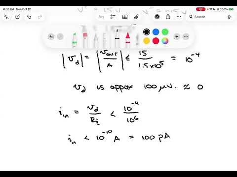
- For an op-amp with open-loop gain 1.5 × 10^5 and a 15 V output limit, the differential input at saturation is about 100 µV, close enough to zero for many ideal-model calculations.
- An input resistance of approximately 1 MΩ combined with a 100 µV differential voltage implies an input current around 100 pA, supporting the ideal assumption of negligible input current.
- A 100 dB common-mode rejection ratio represents a gain ratio of about 10^5, so common signals at both inputs are greatly suppressed but not perfectly eliminated.
- Open-loop op-amp output follows Vout = AVD only until it nears the supply rails; after that, saturation clips the output and enables comparator operation.
- Slew rate, measured in volts per microsecond, limits how quickly an output can change; a fast sinusoidal input can therefore become triangular or otherwise distorted.
- Input offset voltage can create a nonzero output even with shorted inputs; offset-null pins and a potentiometer provide a way to trim that error.
Chapters
- The model retains non-inverting and inverting inputs but adds an input resistance RI across them and an output resistance RO.
- A voltage-controlled voltage source multiplies the differential input voltage VD by open-loop gain A.
- Typical open-loop gain is approximately 10^5 to 10^6, while input resistance is commonly 1 MΩ or higher.
- With A = 1.5 × 10^5 and output limited to about 15 V, VD = Vout/A is roughly 100 µV at the output limit.
- A differential voltage near 100 µV is small enough to approximate the ideal equal-input-voltage assumption in many circuits.
- With RI around 1 MΩ, the estimated input current is below 10^-10 A, or about 100 pA, supporting the ideal zero-input-current approximation.
- An ideal op-amp responds to the difference between its inputs, so a voltage component shared by both inputs cancels.
- Real op-amps can pass some shared signal to the output; CMRR measures rejection as the ratio of open-loop gain to common-mode gain.
- CMRR in decibels is 20 log10(CMRR); a typical 100 dB corresponds to a ratio of about 10^5.
- High CMRR matters when a small signal rides on a larger common offset at both input terminals.
- The linear relation Vout = AVD holds only until the output approaches the positive or negative supply voltage.
- Beyond the supply limits, the output clips near the rails rather than continuing to increase with differential input.
- The steep open-loop gain means even a small differential input can drive the output into saturation.
- Saturation will be used to create comparator behavior in an open-loop op-amp configuration.
- Slew rate describes the maximum speed of output-voltage change and is commonly specified in volts per microsecond.
- If a fast-changing input exceeds the op-amp’s response capability, the output cannot track it and may become distorted.
- A sinusoidal input can produce a more triangular-looking output when the op-amp cannot keep up with its rapid slopes.
- The lecture gives 1 V/µs as an example slew rate and notes that many course circuits use low enough frequencies to avoid this limit.
- A practical op-amp can produce a nonzero output even when its two input terminals are shorted together.
- The resulting input offset voltage may be in the millivolt range and can degrade performance in some applications.
- Offset-null or balance pins let users compensate for the error, typically with a potentiometer.
- Calibration consists of shorting the inputs, monitoring the output, and adjusting the potentiometer until the output approaches zero.
- Ideal assumptions of equal input voltages and zero input current work well for many circuits because practical input differences and currents can be extremely small.
- The practical model adds finite open-loop gain, input resistance, and output resistance, while CMRR, saturation, slew rate, and offset describe further real-device limits.
- A 100 dB CMRR indicates common-mode gain about 100,000 times smaller than differential gain.
- Saturation clamps output near the supply voltages and sets up the next topic, using op-amps as comparators.
Transcript excerpt
0:02 Welcome to ECE 211. This is lecture 16. Last time in lecture 15, we talked about difference amplifier circuits. We also talked about cascaded stages of op-amps. And we concluded the lecture with a practical op-amp model. Today we're going to continue with that practical op-amp model. We'll also talk about some additional characteristics of practical op-amps. And then we're going to move to a topic of using op-amps as comparators. So let's go ahead and just jump right into our practical non-ideal op-amp model. This is the one that we showed last time. Basically what we knew in that case is we still had our two input terminals. We had our non-inverting and inverting terminals. And we still had an output. What we did though is we gave the the insides of the op-amp a little
0:49 more definition. We showed a model that had a large resistor across those two input terminals. We called that RI or input resistance. And then the output was generated by a voltage controlled voltage source. That's this this controlled source here in the middle of the of the model. And what it does is it essentially amplifies that voltage difference across the input terminals. So the gain there is A and A turns out to be rather large for most op-amps. So it's a the parameter that they call the open loop gain. That open loop gain tends to be you know in the order of 100,000 to a million times bigger than the input voltage. So the output increases in magnitude by a factor of five or six orders of magnitude. There's also a
1:37 little bit of resistance in that output path. So that's the output resistance. So RO, that's usually a pretty modest amount. The input resistance we talked about before, that
This is the start of the transcript. Save this video free for the whole transcript, searchable and time-coded.
Related notes
Summary, takeaways, and chapters were generated by AI from the video's transcript and may contain errors. The video belongs to its creator, Roger Green.