NDSU ECE 211 Lecture 15
 Watch on YouTube →
Overview
Roger Green derives a difference amplifier with equal resistor ratios, producing Vout = V2 - V1, then designs and verifies a gain -4 inverting amplifier in CircuitLab. He shows why op-amp stages can be cascaded without loading, contrasts this with resistor dividers that load one another, and introduces a practical op-amp model with finite input and output resistances and large open-loop gain.
Key takeaways
- With the shown equal-resistor difference-amplifier configuration, KVL and the ideal-op-amp condition yield Vout = V2 - V1.
- An inverting amplifier with RF = 2 kΩ and R = 500 Ω has gain -4; with a 100 Ω load, its load-current magnitude is 20 times the input-source current because the op amp supplies additional current.
- CircuitLab time-domain simulation is needed to inspect sinusoidal behavior; a 1-second run with a 1 ms step reveals the gain and inversion that DC analysis cannot show.
- Two buffered inverting stages, each with gain -1/2, produce an overall positive gain of 1/4 without loading one another.
- Two cascaded 1:1 resistor dividers produce Vout = Vin/5, not Vin/4, because the second divider loads the first.
- A practical 741 model can use open-loop gain 2 × 10^5, input resistance 2 MΩ, and output resistance 75 Ω to represent non-ideal behavior.
Chapters
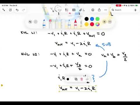
- The difference-amplifier circuit places V1 at the inverting input and V2 at the non-inverting input, with negative feedback.
- Using KVL and the ideal-op-amp condition VA = VB, the non-inverting input voltage is V2/2 for the shown equal-resistor divider.
- Substituting the loop equations gives Vout = V2 - V1.
- For an inverting amplifier, Vout = -(RF/R)VN; choosing RF = 2 kΩ and a target gain of -4 gives R = 500 Ω.
- With the non-inverting terminal grounded, the inverting terminal is a virtual ground, so the input-source current is VN/500 Ω.
- For RL = 100 Ω, the load current is -4VN/100 Ω, whose magnitude is 20 times the input-source current; the op amp supplies the additional output current.
- CircuitLab's basic op-amp component closely approximates an ideal op amp by default; its settings also expose practical parameters such as open-loop gain and slew rate.
- A 1 V DC input with RF = 2 kΩ, R = 500 Ω, and RL = 100 Ω produces a -4 V output, while the simulated currents are 2 mA at the input resistor and 40 mA at the load.
- For a sinusoidal input, DC analysis does not show the changing waveform; time-domain simulation over 1 second with a 1 ms step displays the input and inverted output at four times the amplitude.
- An op-amp stage's high input impedance means the next stage draws negligible input current and does not significantly load the preceding output.
- Each stage can therefore be analyzed as a separate function, then connected in sequence to build a larger circuit operation.
- This buffering property makes op-amp cascades easier to predict than cascades of passive resistor networks.
- A non-inverting amplifier cannot directly provide a gain below one, so Green targets Vout = Vin/4 using two inversions.
- The first inverting stage uses RF = 1 kΩ and R = 2 kΩ to produce -Vin/2.
- A second stage with the same resistor ratio inverts again, yielding Vout = -(-Vin/2)/2 = Vin/4.
- A single divider made from two 1 Ω resistors produces Vout = Vin/2, but two connected dividers do not produce Vin/4.
- Mesh analysis of the combined four-resistor network gives Vout = Vin/5, because the second divider changes the loading on the first.
- Unlike op-amp stages, passive resistor-divider stages are not isolated, so the complete network must be reanalyzed after connection.
- Ideal assumptions of zero input current and equal input-terminal voltages are approximations, not exact descriptions of real op amps.
- A more realistic circuit model can represent finite input resistance, finite output resistance, and amplification of the differential input voltage.
- The model remains an approximation, but it helps assess how closely real devices follow ideal op-amp behavior.
- The practical model places input resistance RA between the non-inverting and inverting terminals, allowing a small nonzero input current.
- A voltage-dependent voltage source generates an output proportional to the differential voltage VD, followed by output resistance RO.
- The model captures finite input and output impedances rather than assuming infinite input resistance and zero output resistance.
- The open-loop gain A multiplies the differential input voltage; typical values cited are approximately 10^5 to 10^6.
- Practical op-amp input resistance is typically in the megohm range or higher, which helps explain why input current is often negligible.
- Output resistance RO is another practical parameter, though Green notes it is less central to the upcoming analysis.
- The 741 example has an open-loop gain of 2 × 10^5, an input resistance of 2 MΩ, and an output resistance of 75 Ω.
- Table 6.3 in the textbook is identified as a reference for typical practical op-amp parameters.
- The next lecture will test how the practical model approximates ideal input-current and equal-terminal-voltage assumptions, then move toward comparators.
Transcript excerpt
0:01 Welcome to NDSU EC211. This is lecture 15. Last time we made an introduction into operational amplifiers. Um we talked about several interesting operational amplifier circuits including the inverting and non-inverting amplifier circuits, a voltage follower configuration, and a summing amplifier. Today we're going to begin by doing one more. Then we'll transition to a quick example, talk a little bit about circuit lab simulation of op amps and then start uh talking about some additional considerations with op amps. So let's go ahead and begin with a difference amplifier which I've gone ahead and drawn the basic configuration on. Um this difference amplifier is one that is intended to take a difference between two inputs. um because we're taking a difference. We're going to put one input
0:47 to the non-inverting terminal and we're going to put one one input to the inverting terminal. Still has that negative feedback configuration that we're used to. And all we want to do is we'd like to go through and analyze this circuit to make sure that the output really does indeed represent a difference between these two. So, we're just looking again at some common configurations using amp op amps to carry out um common and and needed types of operations. So, uh, to begin, I think I'm going to just do a little KVL. So, I'm going to do a loop and follow the voltages around. And the loop that I'm going to pick to begin with is I'm going to follow this V1 and I'm going to go around until I hit the output that returns me to ground. So, there is there is a loop there, right? And I'm just going to go ahead and do my analysis KDL analysis on that first loop. So, um,
1:34 we're going to come down here just a
This is the start of the transcript. Save this video free for the whole transcript, searchable and time-coded.
Related notes
Summary, takeaways, and chapters were generated by AI from the video's transcript and may contain errors. The video belongs to its creator, Roger Green.