NDSU ECE 211 Lecture 19
 Watch on YouTube →
Overview
The lecture develops the capacitor current-voltage relationship from both directions, then uses power and energy calculations to show how a 2 μF capacitor charged linearly to 12 V stores 1.44 × 10⁻⁴ J. It also derives equivalent capacitance for parallel and series networks, explains capacitor construction and polarization, and introduces parasitic resistance and inductance in practical components.
Key takeaways
- For a capacitor, i = C dv/dt and v(t) = v(t₀) + (1/C)∫i(t)dt are complementary relationships, and the integral form requires the initial voltage.
- A 2 μF capacitor charged from 0 V to 12 V over 1 ms draws 24 mA, peaks at 0.288 W, and stores 1.44 × 10⁻⁴ J.
- Capacitors in parallel add directly, while capacitors in series combine by reciprocal sum; two 1 μF capacitors in parallel placed in series with 1 μF yield 2/3 μF.
- The parallel-plate estimate C ≈ εA/d shows that higher dielectric permittivity, greater plate area, and smaller plate spacing increase capacitance.
- Electrolytic capacitors offer high capacitance per volume but require correct polarity; ceramic capacitors are non-polarized and suitable for AC or DC use.
- Real capacitors can exhibit series resistance, series inductance, and dielectric leakage resistance, with parasitics becoming more significant in high-frequency circuits.
Chapters
- A 2 μF capacitor is driven from 0 V to 12 V over 1 ms, producing a predicted constant 24 mA charging current.
- CircuitLab's comma-separated-value source accepts time-voltage pairs and connects them using piecewise-linear interpolation.
- The PWL source uses control points (0, 0), (0.001 s, 12 V), and (0.010 s, 12 V) to ramp and then hold the voltage.
- A 0.0001 s simulation step makes the current pulse look sloped; reducing the step to 0.00001 s resolves the expected square pulse.
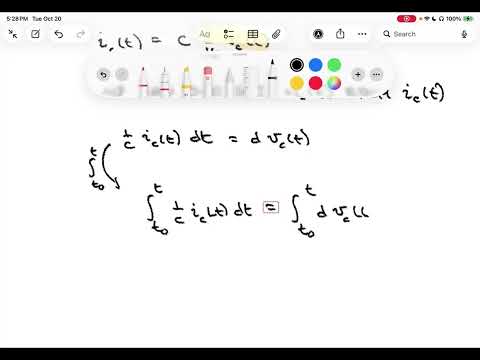
- Starting from iC(t) = C dvc(t)/dt, integration gives vc(t) = vc(t₀) + (1/C)∫ from t₀ to t of iC(τ)dτ.
- The initial capacitor voltage vc(t₀) must be included because current integration alone does not specify the starting voltage.
- The integral relationship complements the derivative form: known voltage gives current, while known current and initial voltage give capacitor voltage.
- Under the passive reference convention, capacitor power is p(t) = v(t)i(t), with positive power indicating absorbed energy and negative power indicating delivered energy.
- Energy accumulated from t₀ to t is the integral of power over time.
- The shortcut w = ½Cv² applies when the initial energy and initial capacitor voltage are both zero; otherwise, account for the initial conditions.
- For the 1 ms linear voltage ramp, the 2 μF capacitor current remains 24 mA while voltage rises from 0 V to 12 V.
- Since p(t) = v(t)i(t), power rises linearly from zero to 12 V × 24 mA = 0.288 W at 1 ms.
- After the ramp, capacitor current returns to zero, so power is zero while the capacitor remains at 12 V.
- Positive power during charging means the capacitor absorbs energy from the source.
- During the ramp, power is p(t) = 288t watts for time t in seconds and 0 ≤ t ≤ 0.001 s.
- Integrating gives w(t) = 144t² joules during the ramp, with zero energy before charging begins.
- For t ≥ 1 ms, accumulated energy remains constant at 1.44 × 10⁻⁴ J, the area under the triangular power pulse.
- The energy curve is quadratic during charging, continuous at 1 ms, and flat after the capacitor reaches 12 V.
- Three parallel capacitors share the same voltage, while their branch currents sum by Kirchhoff's current law.
- Using i = C dv/dt for each branch yields Ceq dv/dt = (C1 + C2 + C3) dv/dt.
- The parallel equivalent is Ceq = C1 + C2 + C3, extending directly to any number of parallel capacitors.
- In a series string, the same current flows through each capacitor, while source voltage is the sum of the capacitor voltages.
- Substituting v = (1/C)∫i(t)dt into Kirchhoff's voltage law gives 1/Ceq = 1/C1 + 1/C2 + 1/C3.
- The reciprocal-sum rule for series capacitors mirrors the parallel-resistor formula, unlike the direct-sum rule for parallel capacitors.
- Two 1 μF capacitors in parallel combine to 2 μF.
- That 2 μF equivalent is in series with the remaining 1 μF capacitor.
- Applying the reciprocal-sum formula gives Ceq = 1/(1/1 + 1/2) μF = 2/3 μF.
- A parallel-plate model estimates capacitance as C ≈ εA/d, where ε represents dielectric permittivity, A is plate area, and d is plate separation.
- With other factors fixed, larger plate area or higher-permittivity dielectric increases capacitance.
- Reducing plate spacing also increases capacitance, although dielectric and manufacturing constraints limit how closely plates can be placed.
- Rolling plate layers into a compact package allows larger effective area without requiring a large flat capacitor.
- An electrolytic capacitor uses a metal plate, a thin oxide dielectric, and an electrolyte serving as the second electrode, enabling high capacitance per volume.
- Electrolytic capacitors are polarized; reversing their intended polarity can degrade the oxide layer, so marked positive and negative terminals matter.
- Ceramic capacitors are non-polarized and can operate in both AC and DC applications.
- Electrolytic capacitor symbols may distinguish the terminals with a straight plate for positive and a curved plate for negative.
- A practical capacitor model can include small series resistance from its metal plates and series inductance associated with magnetic fields from current.
- A parallel resistance models leakage through the dielectric, which is not a perfect insulator.
- These non-ideal parameters are called parasitics; they can often be ignored at low frequencies but matter in some high-frequency applications.
- The ideal capacitor model is a useful approximation, but it omits component effects that may need to be modeled in more demanding circuits.
Transcript excerpt
0:02 Welcome to India shooting CE211. This is lecture 19. Last time we introduced capacitors including a discussion of ideal capacitors and their current voltage relationship. This lecture we're going to continue our discussion of capacitors. Last time we ended with an example where we had a voltage that went from 0 volts and then ramped up linearly to 12 volts over a 1 millisecond interval. And we applied that to a 2 microfarad capacitor and found that the current on that capacitor was a pulse of current 24 milliamps over that 1 millisecond duration where the voltage was actively changing. We're going to take just a few minutes and verify this in Circuit Lab including introducing the use of something called a comma separated value.
0:50 Source in Circuit Lab. Okay, we're over in Circuit Lab and we're going to simulate this charging capacitor. I want to take a 2 microfarad capacitor and I want to charge it up to 12 volts but I want that 12 volts to ramp up from 0 to 12 volts over a 1 millisecond duration. Our regular DC voltage source isn't going to do it and so we need something more flexible and it turns out Circuit Lab gives us a flexible voltage source also a current source that is called a CSV source. So I've gone ahead and put that into my circuit. CSV just stands for comma separated value. And what it allows you to do is it allows you to put in time voltage pairs. So a voltage at a particular time, another
1:37 voltage at another time, another voltage at another time and it will connect those control points with a straight line. And you can create very sophisticated, very customized waveforms in this way. You can use very long lists in our particular application we're
This is the start of the transcript. Save this video free for the whole transcript, searchable and time-coded.
Related notes
Summary, takeaways, and chapters were generated by AI from the video's transcript and may contain errors. The video belongs to its creator, Roger Green.