Math 1153 - 20 October 2026 - Chapter 7

Overview

The lecture develops least-squares regression from calculator setup through interpretation, prediction, and residual analysis. Using algae growth data, Mike Jacobsen obtains the line ŷ = -0.85 - 0.91x, interprets its intercept and slope in context, predicts a growth rate of -2.67 for two grazers, and calculates a residual of 0.47; a second example models readings from mini and standard Wright peak flow meters.

Key takeaways

A least-squares regression line minimizes the sum of squared residuals, where each residual is observed Y minus predicted ŷ.
For the algae study, the fitted model ŷ = -0.85 - 0.91x predicts a net growth rate of -2.67 when two Daphnia magna grazers are used.
The algae-model slope means each additional grazer is associated with a predicted decrease of 0.91 in net growth rate; a negative slope requires the word decreases in the interpretation.
For two grazers, the observed growth rate of -2.2 minus the predicted rate of -2.67 gives a positive residual of 0.47, placing the data point above the regression line.
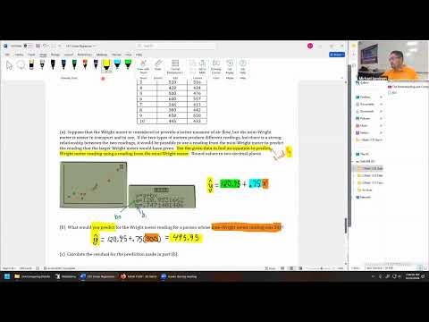
The 10-person peak-flow study models standard Wright meter readings from mini Wright meter readings with ŷ = 120.95 + 0.75x.
A mini Wright reading of 500 produces a predicted standard Wright reading of 495.95, even though the recorded standard-meter value in the study was 476.

Chapters

0:00 Exam Note Sheets, Grading, and Returning Exam Materials

Mike Jacobsen says he will include students’ Exam 2 note sheets when downloading and returning scanned exams, addressing a problem with testing centers retaining the notes.
He plans to begin grading Exam 2 on Friday, aiming to finish Friday or Saturday rather than the late-Sunday cutoff.

2:39 Course Schedule and Chapter 7 Linear Regression

Week 9 marks the semester’s second half; the class expects Exam 3 around weeks 12 to 13, followed by Thanksgiving and a review-focused close week.
Chapter 7 covers linear regression, while the upcoming Chapter 6 quiz revisits earlier scatterplot and correlation skills.

4:31 Least-Squares Regression Minimizes Squared Errors

For each scatterplot point, the residual is the observed response Y minus the line’s predicted response ŷ = A + BX.
The least-squares regression line is the line that minimizes the sum of squared residuals across all observations.
The calculator supplies the intercept A and slope B, avoiding the full hand calculation.

8:32 Algae Growth Study: Grazers as the Explanatory Variable

The first example studies whether Daphnia magna grazers control an invasive algae’s net growth in test tubes.
Number of grazers is the explanatory variable on the x-axis; net growth rate is the response variable on the y-axis.
Negative growth rates indicate reduced algae abundance, with the example describing growth rates of -1.9 for one grazer and -4.3 for four.

13:02 TI Calculator Regression Output and the Algae Model

Enter grazer counts in calculator list L1 and net growth rates in L2, then use STAT, CALC, and option 8, A + BX.
The calculator returns an intercept of -0.85 and slope of -0.91, giving ŷ = -0.85 - 0.91x.
The correlation is negative and described as strong, consistent with the downward trend as grazer count increases.

20:21 Interpreting the Regression Y-Intercept in Context

A y-intercept represents the predicted response when the explanatory variable X equals zero.
For the algae model, zero grazers predicts a net growth rate of -0.85.
Jacobsen’s interpretation template names the x-variable condition, then the predicted y-variable value; whether zero is meaningful depends on the study context.

26:05 Interpreting the Slope as Change in Growth per Grazer

The slope -0.91 is a rise-over-run rate: change in net growth rate divided by change in number of grazers.
A contextual interpretation states that as the number of grazers increases by one, the predicted net growth rate decreases by 0.91.
The direction word, such as increases or decreases, must match the slope’s sign; the x-variable is the explanatory variable and the y-variable is the response.

38:01 Predicting Algae Growth for Two Grazers

Substitute x = 2 into ŷ = -0.85 - 0.91x to predict a net growth rate of -2.67.
The observed value for two grazers is -2.2, which differs from the model prediction because the data point does not lie exactly on the regression line.
A prediction from the regression line estimates the response, rather than repeating the observed data value.

41:37 Residuals: Observed Minus Predicted

A residual is calculated as observed Y minus predicted ŷ; for two grazers, -2.2 - (-2.67) = 0.47.
A positive residual means the observed scatterplot point is above the regression line; a negative residual means it is below.
The least-squares line minimizes the sum of squared residuals, not the sum of raw residuals.

50:48 Comparing Mini and Standard Wright Peak Flow Meters

The second study compares air-flow readings from a portable mini Wright meter and a larger Wright meter for 10 people.
The larger Wright meter is treated as the better measure, while the mini meter is more portable; the goal is to predict standard-meter readings from mini-meter readings.
The mini Wright reading is the explanatory variable X, and the standard Wright reading is the response variable Y.

59:11 Entering Meter Data and Fitting the Regression Line

After entering mini-meter readings in L1 and Wright-meter readings in L2, use ZoomStat to display the scatterplot.
The plotted readings show a strong positive linear association, supporting prediction from the portable instrument to the larger device.
STAT, CALC, option 8 gives the model ŷ = 120.95 + 0.75x, rounded to two decimal places.

1:05:15 Predicting a Wright Meter Reading from 500

For a mini Wright reading of 500, substitute x = 500 into ŷ = 120.95 + 0.75x to get a predicted standard-meter reading of 495.95.
The observed standard Wright reading at 500 on the mini meter is 476, illustrating that predictions need not equal individual observations.
The difference between 476 and 495.95 is a residual; the lecture defers its calculation in this example to the next class.

1:08:15 Wrap-Up and Next Class

Once the regression equation is obtained, later questions use ordinary calculator arithmetic rather than additional specialized regression functions.
The class will continue the meter example on Thursday, finish the notes, and then move to Chapter 10.

Summary, takeaways, and chapters were generated by AI from the video's transcript and may contain errors. The video belongs to its creator, Mike Jacobsen.