MAT291: Lecture 24 - Vector Identities and the Fundamental Theorems
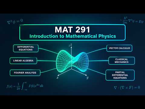
Overview
Parinaz Naseri introduces vector calculus through two identities, curl of a gradient equals zero and divergence of a curl equals zero, then connects them to conservative, source-free fields and Helmholtz decomposition. She explains the divergence theorem and Stokes' theorem with physical interpretations and worked examples, including a cube whose total flux is 3 and a unit-circle circulation that evaluates to π.
Key takeaways
- For a scalar function with continuous second partial derivatives, curl(grad F) = 0 because the mixed partial derivatives cancel component by component.
- For a sufficiently smooth vector field, div(curl F) = 0, so curl-generated fields have no net local sources or sinks.
- The scalar Laplacian is div(grad F), which expands in three dimensions to Fxx + Fyy + Fzz.
- On suitable domains, Helmholtz decomposition separates a vector field into a gradient component grad φ and a curl component curl A, corresponding to curl-free and divergence-free parts.
- The divergence theorem converts total outward flux through a closed surface into the volume integral of divergence; for the field (x², y², z²) on the unit cube, both sides equal 3.
- Stokes' theorem equates boundary circulation with integrated curl, provided the boundary direction and surface normal obey the right-hand rule; the unit-circle example evaluates to π.
Chapters
- Naseri frames vector calculus as a tool for operating on vector fields such as electric and magnetic fields.
- She highlights applications in electromagnetics, quantum computing, and later engineering courses including EC 221 and EC 320.
- The lecture prioritizes conceptual explanations and examples over covering every slide.
- The gradient of a scalar function points normal to its level curves, so it has no circulation around closed paths in the illustrated smooth-field setting.
- Applying curl to grad F produces pairs of mixed second partial derivatives, such as Fzy and Fyz.
- Schwarz's theorem makes those mixed partials equal when the second derivatives are continuous, causing the curl components to cancel.
- Naseri interprets curl as local circulation: taking the divergence of a curl gives zero for sufficiently smooth vector fields.
- The component calculation differentiates the curl components and cancels mixed partial derivatives using the same equality of continuous mixed partials.
- A curl field is therefore divergence-free, also described as source-free or solenoidal; a gradient field is curl-free, or irrotational.
- The scalar Laplacian is written as ∇²F = div(grad F), rather than as curl of the gradient.
- Expanding the operator gives the sum of second partial derivatives: Fxx + Fyy + Fzz.
- Naseri distinguishes the scalar Laplacian from the vector Laplacian, which is not covered in this lecture.
- Helmholtz decomposition represents a general vector field as a curl-free part plus a divergence-free part.
- On a suitable domain, the curl-free component can be written as grad φ, while the source-free component can be represented as curl A.
- Naseri connects the scalar potential φ to electric or gravitational potential and describes the vector potential A as useful in transient-field applications.
- The divergence theorem equates the outward flux integral over a closed surface S with the volume integral of div F over the enclosed region.
- A closed surface is required because it encloses a volume; its shape can vary, including a sphere or box.
- The volume integral sums local sources and sinks, while internal contributions cancel so the net result is measured by flux through the boundary.
- Using Gauss's law, Naseri relates div E to volumetric charge density ρv divided by permittivity ε.
- Integrating ρv over the enclosed volume gives total charge Q, linking electric flux through a closed surface to the charge it contains.
- Positive and negative charges can cancel: if their net enclosed charge is zero, the total outward electric flux is zero.
- For F = (x², y², z²) on the unit cube 0 ≤ x,y,z ≤ 1, the divergence is 2x + 2y + 2z.
- Integrating the divergence over the cube gives 3, with each of the three coordinate terms contributing 1.
- The flux through the three faces at x=0, y=0, and z=0 is zero; the opposite faces each contribute 1, giving total flux 3.
- A face integral uses two surface coordinates, such as dx dy on the top face z=1, because z is fixed there.
- Stokes' theorem equates circulation of F around a closed boundary curve C with the surface integral of curl F over a surface bounded by C.
- Different surfaces, such as a flat disk or a dome, give the same boundary circulation when they share the same boundary and the field is well behaved.
- The curve direction and surface normal must follow the right-hand rule; reversing one requires reversing the other to preserve the sign.
- For F = (y², x, z²) on the unit circle x² + y² = 1 in z=0, Naseri uses r(t) = (cos t, sin t, 0) for 0 ≤ t ≤ 2π.
- The counterclockwise parametrization gives tangent vector r′(t) = (−sin t, cos t, 0) and upward normal z-hat.
- Substituting the curve into F and taking the tangent dot product gives −sin³t + cos²t; integration over 0 to 2π yields π.
- Naseri leaves the surface-integral checks for a flat disk and a hemisphere as follow-up work.
Transcript excerpt
0:00 Good morning, everyone. So, today we are going to go deep into the topic that is called vector calculus. Okay? If you're thinking about a career or a research in electromagnetics or quantum computing, this is going to be your tool, basically. So, we are away from scalar functions and deep into the vector fields, electric field, magnetic fields, and all kinds of other fields that you can imagine. This is the tool to basically operate calculations on them. Okay? Today we are going to go through some identities that are called vector
0:49 identities and the fundamental theorems. Actually, today's lecture and the next two or three ones are very, very important because they provide you with the tool that you will need at least for EC 221 that is a mandatory course. Obviously, if you take other courses, as I mentioned in quantum computing or quantum related or EC 320, this is also going to come back in your courses as well. Okay? So, we have a tight agenda today. We might not cover everything that you see on the slides, but it's okay. I prefer to go deeper and explain things conceptually first and then we work through some examples. If you finish them all, good. If we don't, then we
1:37 move to we cover them in the next lecture. Okay? So, don't get stressed about the fact that we are not covering everything you see on the slides today. Okay, the vector identities. The slide looks very crowded just because I couldn't get animation working on what is handwritten. So, for a second, just look on the left side of the slide, which mentions the curl of a gradient is always zero. Okay? So we mentioned before that gradient is applied on a scalar functions. Okay? So let's imagine that
This is the start of the transcript. Save this video free for the whole transcript, searchable and time-coded.
In this course
Related notes
Summary, takeaways, and chapters were generated by AI from the video's transcript and may contain errors. The video belongs to its creator, Parinaz Naseri.