MAT 291: Lecture 22 - Circulation Flux, Curl & Divergence
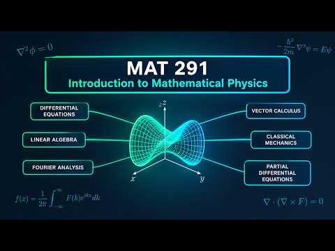 Watch on YouTube →
Overview
The lecture develops curl and divergence from circulation and flux by measuring each quantity on an infinitesimal region, then normalizing by area in 2D or volume in 3D. It derives the 2D formulas, explains curl as a vector and divergence as a scalar, and applies both to the fields (x² − y², 2xy) and (x²y, y²z, z²x), including their values at (1, 2, 3).
Key takeaways
- In 2D, local circulation per unit area is ∂Fᵧ/∂x − ∂Fₓ/∂y, with positive values corresponding to counterclockwise circulation under the stated orientation convention.
- Divergence measures local outward flux: positive values indicate a source, negative values indicate a sink, and zero means no net local expansion or contraction.
- For the field (x² − y², 2xy), divergence is 4x and curl is 4y, so source or sink behavior changes across the y-axis while rotational direction changes across the x-axis.
- In 3D Cartesian coordinates, curl is computed by the determinant arrangement of unit vectors, partial derivatives, and field components; its output has three components.
- For F = (x²y, y²z, z²x) at (1, 2, 3), curl is (−4, −9, −1) and divergence is 22, showing how curl and divergence provide separate local descriptions of rotation and flux.
Chapters
- Circulation along a curve is the integral of F · T ds, where T is tangent to the curve and ds is a length element.
- Curve flux uses F · n ds to measure the component crossing the curve rather than moving along it.
- For a counterclockwise boundary in the plane, the outward normal points to the traveler's right; reversing orientation changes the integral's sign.
- Dividing circulation or flux by the enclosed area removes dependence on the size of the test region and isolates behavior near a point.
- The field F = (x, y) points radially outward and illustrates source-like flux without local swirl.
- The field F = (−y, x) is tangent to circles around the origin and illustrates circulation without radial flux.
- At a point, 2D curl is obtained by taking circulation around a shrinking closed curve and dividing by its enclosed area.
- The resulting value depends on both the vector field and the location where the small region is centered.
- A small rectangle provides a simpler derivation than a circle because its four tangent directions align with the Cartesian axes.
- For a counterclockwise rectangle with side lengths dx and dy, the four edge contributions combine into differences in the vector components Fₓ and Fᵧ.
- Dividing the circulation by the rectangle's area dx dy yields ∂Fᵧ/∂x − ∂Fₓ/∂y.
- The derivation approximates the field as nearly constant on each very short edge, then uses component differences to obtain partial derivatives.
- In 3D, curl is a vector whose components represent circulation around small loops in the coordinate planes.
- Divergence is net outward flux per unit area in 2D or per unit volume in 3D, and is a scalar rather than a vector.
- Positive divergence indicates source-like behavior, negative divergence indicates sink-like behavior, and 3D divergence is ∂Fₓ/∂x + ∂Fᵧ/∂y + ∂F_z/∂z.
- For Fₓ = x² − y² and Fᵧ = 2xy, divergence is ∂Fₓ/∂x + ∂Fᵧ/∂y = 2x + 2x = 4x.
- The 2D curl is ∂Fᵧ/∂x − ∂Fₓ/∂y = 2y − (−2y) = 4y.
- Positive divergence for x > 0 marks source-like behavior and negative divergence for x < 0 marks sink-like behavior; positive curl for y > 0 indicates counterclockwise rotation.
- For a field confined to the xy-plane, its 2D curl points along the z-axis, so the scalar 4y is written as the vector 4y k̂.
- The right-hand rule maps counterclockwise circulation in the xy-plane to positive z and clockwise circulation to negative z.
- The same orientation convention applies to interpreting magnetic-field circulation and dipole direction.
- For F = (x²y, y²z, z²x), the Cartesian curl setup uses rows x̂, ŷ, ẑ; ∂/∂x, ∂/∂y, ∂/∂z; and Fₓ, Fᵧ, F_z.
- Expanding the determinant gives curl F = (−y², −z², −x²), while divergence is 2xy + 2yz + 2zx.
- At P = (1, 2, 3), curl F = (−4, −9, −1) and divergence is 22, indicating source-like behavior at that point.
- The nabla operator applied to a scalar function produces its gradient, a vector normal to the function's level curves.
- Nabla crossed with a vector field produces curl, which is a vector; nabla dotted with a vector field produces divergence, which is a scalar.
- The lecture closes by distinguishing positive, negative, and zero curl or divergence as rotational, source-or-sink, or locally neutral behavior.
Transcript excerpt
0:01 Good morning everyone. Good morning. So, so far what we've talked about is circulation and flux of vector fields on curves, right? And surfaces. So, circulation was only defined on curves. Flux we define it both on curves and surfaces. In fact, for circulation, usually it just makes sense to consider them on boundaries because circulation, even if you consider it at a surface, you're exactly thinking of a boundary on that surface as well. But for a surface flux through surface can happen more naturally than a curve just physically practically that's that's what's happening in most
0:51 applications that flux is happening through uh surfaces circulation happens over curves. But today we're going to take this further. We are going to use the definition of circulation and flux to actually come up with something very important. Two things actually very important about vector fields. Okay. So just to review, we talked about circulation as the curve integral right or single variable integral of f dot t ds where ds here was a length element. Remember that we use t as a fourth
1:50 variable and we actually define ds in terms of something dt which was the speed of the movement on that curve dt. Then we also define a flux on a curve. And that way we said for this one we said whatever that doesn't circulate over the curve whatever of the vector that doesn't circulate over the curve it passes through the curve. And then in order to calculate that we need a vector or a unit vector that is normal to the curve not tangential to it. So that's why we projected f into the n hat by calculating f nhat and then reuse
2:41 that ds which was the lens element. Correct. We defined some conventions
This is the start of the transcript. Save this video free for the whole transcript, searchable and time-coded.
Related notes
Summary, takeaways, and chapters were generated by AI from the video's transcript and may contain errors. The video belongs to its creator, Parinaz Naseri.