Lecture 18: Kondo impurity model
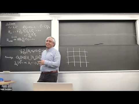 Watch on YouTube →
Overview
Subir Sachdev concludes the t-J mean-field discussion of cuprate superconductivity, deriving how nearest-neighbor singlet pairing on a square lattice can produce d-wave nodes and anisotropic Dirac-like Bogoliubov excitations. He then introduces the Kondo impurity model, relates its anomalous low-temperature resistance to renormalization-group growth of antiferromagnetic exchange, and begins an exactly solvable resonant-level model as preparation for later calculations.
Key takeaways
- In the t-J mean-field treatment, replacing holons by their condensate value √P renormalizes electron hopping, but the approximation depends on relaxing a local constraint that Sachdev argues must be taken seriously.
- Nearest-neighbor d-wave pairing on a square lattice has Δk proportional to cos(kx) − cos(ky); its gap zeros intersecting the Fermi surface produce four cuprate nodes with anisotropic Dirac velocities vF and vΔ.
- Photoemission can reveal nodal dispersion but not the pairing phase; phase-sensitive Josephson tunneling by Tsuei and Kirtley provided direct evidence for d-wave symmetry.
- For a Kondo impurity, weak antiferromagnetic exchange grows under reduction of the energy cutoff, whereas ferromagnetic exchange flows toward zero, explaining the low-temperature increase in impurity scattering.
- The weak-coupling Kondo RG predicts an upturn but not the eventual saturation; Wilson’s numerical renormalization group addresses the strong-coupling regime.
- A single Kondo impurity changes bulk observables only through a non-extensive correction: the bulk can renormalize the impurity, while the impurity does not renormalize the bulk electron band.
Chapters
- Sachdev announces class presentations, a final problem set on the Kondo effect, and an online class on Thursday.
- He frames the lecture as a transition from t-J mean-field theory to the Kondo impurity model.
- The t-J mean-field approach has had some success at higher doping, but has not adequately explained the low-doping region near the Mott insulator.
- The projected t-J Hilbert space allows three states per site: spin up, spin down, or empty.
- Sachdev writes the electron operator as a product of a spinon and a holon, with a local constraint enforcing the allowed states.
- Doping introduces a hopping term of order T, while the exchange term retained at next order has J = 4T²/U.
- A common approximation replaces each holon operator H with its mean value, the square root of the hole density P.
- This assumption renormalizes electron hopping and yields an effective electron t-J Hamiltonian.
- Sachdev stresses that the model is reasonable only if its local constraints are treated seriously; replacing holons by their average is the less controlled step.
- The exchange interaction is decoupled in a spin-singlet pairing channel on square-lattice bonds.
- Bond pairing amplitudes Δij define a quadratic BCS-type Hamiltonian that can be diagonalized for a trial wave function.
- Minimizing the expectation value of the original Hamiltonian over these trial states gives a variational procedure; its minimum agrees with the self-consistent Hartree-Fock saddle point.
- For spin-singlet pairs, the spin wave function is antisymmetric, so fermion antisymmetry requires the spatial pairing amplitude to be symmetric.
- On a square lattice with translation symmetry, the nearest-neighbor amplitudes can be represented by Δx and Δy.
- The two key rotation-symmetric patterns are Δx = Δy, called extended s-wave, and Δx = −Δy, called d-wave.
- The d-wave pattern changes sign under a 90-degree rotation, but physical quantities remain rotation invariant because the order parameter’s overall phase change does not alter them.
- Extended s-wave pairing has the same square-lattice symmetry as on-site s-wave pairing, but nearest-neighbor pairing avoids the costly double occupancy penalized by the Hubbard repulsion.
- For the usual nearest-neighbor t-J model, the d-wave solution is lowest in energy; more complicated Fermi surfaces, including those discussed for nickelates, can make extended s-wave competitive.
- Nearest-neighbor hopping becomes a momentum-dependent dispersion, while bond pairing gives Δk proportional to Δx cos(kx) + Δy cos(ky).
- For d-wave pairing, Δx = −Δy, so Δk is proportional to cos(kx) − cos(ky).
- A Bogoliubov transformation diagonalizes the quadratic Hamiltonian into spin-rotation-invariant quasiparticles with energy Ek = √(ξk² + |Δk|²).
- The d-wave gap vanishes along kx = ±ky; intersections of those lines with the Fermi surface yield four nodal points in the usual cuprate geometry.
- Near each node, the excitation energy is Dirac-like: E(q) = √(vF²q⊥² + vΔ²q∥²), with distinct velocities normal and parallel to the Fermi surface.
- Unlike graphene’s ordinary electron Dirac cones, these are Bogoliubov quasiparticles in a gapless superconductor and couple differently to electromagnetic fields.
- Photoemission measurements of nodal quasiparticle dispersion provided strong early evidence for d-wave pairing in cuprates.
- Nodal points require both a zero of Δk and a Fermi surface crossing; strong pairing or a changed chemical potential can remove the nodes.
- Phase-sensitive Josephson tunneling experiments by C. C. Tsuei and J. R. Kirtley tested the pairing phase directly and confirmed d-wave symmetry.
- Sachdev notes that this mean-field framework can describe some higher-doping behavior but does not explain why the cuprates have a high transition temperature.
- The t-J model combines spin-liquid physics and a Fermi surface arising from the same electrons, making their interaction especially complex.
- The Kondo impurity model offers a simpler setting: localized spins and conduction electrons come from distinct degrees of freedom or bands.
- For a clean metal such as copper, the low-temperature Pauli spin susceptibility is nearly constant and is proportional to the single-spin density of states at the Fermi energy.
- Adding dilute manganese impurities to copper produces a resistivity minimum, unlike the ordinary decrease in scattering as temperature falls.
- The impurity contribution to magnetic susceptibility rises at low temperature and eventually saturates around the Kondo temperature.
- Jun Kondo explained the resistivity upturn perturbatively; Kenneth Wilson’s numerical renormalization group later clarified the strong-coupling regime and low-temperature saturation.
- A manganese impurity supplies a localized magnetic moment, modeled in the simplest case as a spin-1/2, while copper supplies mobile conduction electrons.
- The Kondo exchange couples the impurity spin to the conduction-electron spin density at the impurity site, conventionally set to R = 0.
- Spin exchange during successive electron-scattering events creates interference, so the impurity is a dynamical degree of freedom rather than an ordinary static scatterer.
- The single-impurity treatment assumes impurities are dilute and independent; at higher concentration, interactions between impurity spins can lead to spin-glass behavior.
- The Kondo problem contains both a degenerate impurity spin and many conduction-electron states near the Fermi level, making low-energy processes important.
- An RG step removes thin shells of high- and low-energy electron states around the bandwidth using a canonical transformation.
- Unlike transforming the Hubbard model into a different low-energy model, the Kondo transformation reproduces the same form of Hamiltonian with altered parameters.
- Anderson and Yuval recast the perturbative scaling structure as an RG flow, building on Kondo’s perturbative result.
- At weak coupling, the exchange flow is quadratic in J_K and proportional to the density of states; the precise coefficient depends on conventions.
- For antiferromagnetic J_K > 0, reducing the cutoff increases the coupling, while ferromagnetic J_K < 0 flows toward zero.
- The growing antiferromagnetic coupling explains why impurity scattering strengthens as temperature falls, producing the Kondo resistance upturn.
- The weak-coupling flow eventually becomes unreliable as J_K grows, so it cannot by itself explain low-temperature saturation; Wilson’s numerical RG includes the strong-coupling behavior.
- A single impurity gives a non-extensive correction: the bulk electron dispersion and density of states do not flow, but the bulk can renormalize the impurity.
- Sachdev compares coupling flows with quantum chromodynamics, where strong low-energy coupling produces confinement and weak high-energy coupling gives asymptotic freedom; the Kondo impurity’s high-temperature limit instead has a free local spin with Curie susceptibility.
- The exactly solvable resonant-level model replaces the local spin with an impurity state of energy ED that hybridizes with conduction electrons through hopping W.
- When ED lies near the Fermi level, the impurity state can strongly affect scattering; Sachdev leaves its Green’s-function calculation for the next lecture.
Transcript excerpt
0:12 Finish. That's it. Couple of announcements. Uh-huh. Oh, what is that? Thanks for signing up for the presentation. Looks like everyone has signed up. Uh I'll get back to you on your titles and if you haven't put your titles, okay. Uh put it in at some point. Um I promised there'd be one more problem set. Um I've written part of it and I don't know the next part of it will be on the condo effect. That's why I haven't given it out to you yet. Uh it'll be due after your presentation sometime before my grades are due. Uh so don't be in a rush on that. Uh And another announcement, uh
1:01 this Thursday, the day after tomorrow, um the class will be online. I I won't be here. I'll be at a conference. Uh and that's the last online talk. Uh I'll be back after that. >> [clears throat] >> All right. So, today I want to wrap up the discussion of the TJ model, at least uh in the standard mean field theory, which is the foundation of really hundreds of papers, if not thousands, uh in the literature with the hope of understanding uh high temperature superconductivity. Uh and it's fair to say, as a disclaimer, that it it sort of seems to work in the region where TC is lower high doping.
1:48 Uh but in the interesting region at low doping near the Mott insulator, uh this approach really hasn't been that successful. And uh Um eventually, towards the end of the course, I will uh back to to some more recent approaches which look quite promising. Okay, so this is the the standard approach. Um so, you do you start with a Mott insulator, which is an antiferromagnet. You dope it. Uh and then you allow for only three
This is the start of the transcript. Save this video free for the whole transcript, searchable and time-coded.
Related notes
Summary, takeaways, and chapters were generated by AI from the video's transcript and may contain errors. The video belongs to its creator, Subir Sachdev.