Lecture 13: Linear least squares
 Watch on YouTube →
Overview
Burton Ma derives ordinary linear least squares by expressing observations as y = Xw + ε, defining residuals, and minimizing their squared sum. He constructs design matrices for estimating a repeated measurement, fitting lines and polynomials, then derives the normal equation w = (XᵀX)⁻¹Xᵀy; for repeated direct measurements, this solution reduces to their average.
Key takeaways
- A linear least-squares model represents m observations and n unknown parameters as y = Xw + ε, with the design matrix encoding each observation's predictors.
- A line fit has design-matrix rows [xᵢ, 1], while a quadratic fit uses [xᵢ², xᵢ, 1]; both are linear in their unknown coefficients.
- Ordinary least squares minimizes the sum of squared residuals, and its gradient yields the normal equation XᵀXw = Xᵀy.
- If XᵀX is invertible, the least-squares solution is w = (XᵀX)⁻¹Xᵀy.
- For normally distributed measurement noise with mean zero, Gauss's result establishes least squares as an optimal estimator under that assumption.
- Repeated direct measurements of a single quantity have an all-ones design matrix, making their least-squares estimate exactly the arithmetic mean.
Chapters
- Least squares combines multiple observations to estimate a model, such as a line fitting measured points (xᵢ, yᵢ).
- A residual is the vertical difference between an observation and the model prediction; orthogonal regression instead measures perpendicular distances.
- Minimizing squared residuals is more tractable than minimizing absolute residuals, the latter being associated with L1 regression.
- A linear model maps a parameter vector w in ℝⁿ to observations in ℝᵐ using a matrix X with m rows and n columns.
- The unknown entries of w are model parameters; a straight line has two, its slope and y-intercept.
- Estimating n parameters requires enough independent equations, and fitting a line requires observations at at least two distinct x-values.
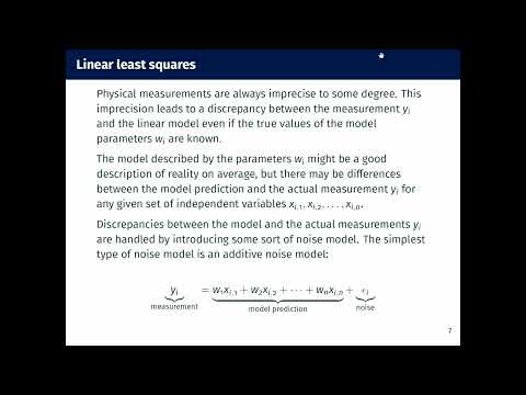
- Measurements differ from model predictions because of noise, represented as additive error εᵢ with an assumed average of zero.
- The observation model becomes y = Xw + ε, where y contains m measured values and w contains the model parameters.
- The design matrix X has m observation rows and n parameter columns; its entries encode the chosen independent variables.
- For repeated measurements of one person's height, the unknown height is a single parameter w₁.
- Each measurement observes the same parameter plus its own noise, so the design matrix is an m-by-1 column of ones.
- This simple setup shows how direct measurement can be represented as a least-squares problem.
- For a line, each design-matrix row is [xᵢ, 1], and the two parameters are the slope and y-intercept.
- A quadratic fit uses row [xᵢ², xᵢ, 1] and three coefficients; adding columns for higher powers fits cubic and higher-degree polynomials.
- These models remain linear least-squares problems because they are linear in the unknown coefficients, even when the fitted curve is nonlinear in x.
- For observation i, the residual is yᵢ − xᵢᵀw; collecting all m residuals gives r = y − Xw.
- Minimizing the sum of absolute residuals is called least absolute deviations or least absolute errors, and is harder to solve analytically.
- Ordinary least squares instead minimizes the sum of squared residuals, sometimes written with a factor of 1/2 to simplify differentiation.
- Least-squares history includes Adrien-Marie Legendre's 1805 publication and Carl Friedrich Gauss's later claim that he had solved the problem earlier.
- Gauss showed that least squares is optimal under the assumption that measurement errors are normally distributed with mean zero.
- Ma begins a broader derivation for predictions f(xᵢ, w), which can be nonlinear in the parameters, by differentiating the sum of squared residuals.
- With residual rᵢ = yᵢ − fᵢ(w), differentiating rᵢ² produces 2rᵢ times the gradient of rᵢ.
- The measured value yᵢ is constant with respect to w, so the derivative comes from the model function fᵢ.
- For a linear model fᵢ = xᵢᵀw, its gradient with respect to w is xᵢ, the i-th row of X written as a column vector.
- Stacking the row vectors xᵢᵀ and the observations yᵢ converts sums of vector terms into matrix products.
- The gradient of the squared-error objective, with the 1/2 factor, becomes −Xᵀy + XᵀXw.
- Setting this gradient to zero gives the normal equation XᵀXw = Xᵀy.
- When XᵀX is invertible, the least-squares parameters are w = (XᵀX)⁻¹Xᵀy.
- For m repeated measurements of one quantity, X is a column of ones, so XᵀX = m and the solution is (y₁ + ··· + yₘ)/m.
- The arithmetic mean is therefore the least-squares estimate for repeated direct measurements under this model.
Transcript excerpt
0:01 All right. Uh good morning everybody. Uh welcome back from reading week. Uh so to begin things off uh there was um there was some p not well there were some sample test questions again posted to on uh last night while I was doing the solutions up for them. Um I discovered that there was a typo in question five. the equation for the sphere is incorrect. Well, it's not incorrect, but it was the equation of a sphere for of radius zero. So, it was the equation of a point. Um, so I fixed that. Uh, and question 6A was very slightly rewarded. Um, so if you're uh looking at the sample questions, uh, they've been updated. Uh, also the
0:50 solutions for the sample questions are available now. Um, and I'll get around to posting the solutions for the homework, I guess, for week the third homework or the fourth home. I don't remember which one now. Uh, later uh today or tomorrow. All right. So, the topic of today's lecture is uh the le squares method uh including the linear and nonlinear um whoops cases. All right. So I took just took a look at what you did in 271 or at least what the Dr. Ellis's notes say you did in 271. I don't know if you actually did them in 271. Um and so what you were taught in 271 was the linear case for le squares. Uh and in specifically uh you were taught the way to do it. Uh you were
1:39 taught like subtract the mean and do some other stuff. Um I'm going to show you the other way or a different way of uh approaching the problem that also generalizes to the nonlinear case. Uh so often the way this problem is
This is the start of the transcript. Save this video free for the whole transcript, searchable and time-coded.
In this course
Related notes
Summary, takeaways, and chapters were generated by AI from the video's transcript and may contain errors. The video belongs to its creator, Burton Ma.