L22 Phase Kick Back and Shor's Algorithm Part II
Overview
Hiu-Yung Wong connects quantum phase estimation to Shor’s algorithm, first showing how phase kickback transfers a controlled phase into a control qubit’s superposition. The lecture then explains how Shor reduces factoring to finding the period of a^x mod N, works through factoring 21 using a = 11 and period r = 6, and derives the algorithm’s register preparation, quantum-oracle evaluation, QFT, and measurement-induced periodic state.
Key takeaways
- A unitary operator’s eigenvalues have magnitude one, so phase estimation can represent each eigenvalue as e^(iθ) and estimate φ = θ/(2π).
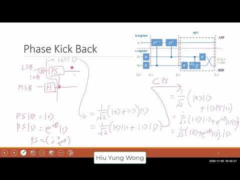
- Phase kickback requires superposition: a controlled phase on target |1⟩ gives the control branches a relative phase e^(iθ), while the target stays unchanged.
- For N = 21 and a = 11, the modular sequence has period 6, and gcd(11^3 + 1, 21) = 3 plus gcd(11^3 − 1, 21) = 7 recover the factors.
- Shor’s circuit encodes f(x) = a^x mod N in a reversible XOR oracle, then applies the QFT to extract periodic structure rather than reading every function value.
- Measuring the function register selects a residue shared by multiple inputs; those inputs remain separated by the period, as residue 1 leaves x = 0, 6, 12, and later repeats.
- The lecture’s register estimate is 3n logical qubits for an n-bit modulus; its N = 21 example uses 15 logical qubits, while fault-tolerant physical-qubit overhead can be much larger.
Chapters
- For a unitary U and eigenvector |λ⟩, U|λ⟩ = λ|λ⟩ and U†U = I imply |λ|²⟨λ|λ⟩ = ⟨λ|λ⟩.
- Since an eigenvector is nonzero, its eigenvalue has magnitude 1 and can be written e^(iθ).
- Quantum phase estimation targets the normalized phase φ = θ/(2π), rather than estimating θ directly.
- The standard phase-estimation circuit combines Hadamard gates, controlled applications of U, and a quantum Fourier transform.
- The controlled operations use powers U^(2^j), allowing their accumulated phase information to encode binary digits of φ.
- For U = Z, the circuit uses controlled powers of Z to reveal the eigenvalue phase.
- A Hadamard gate prepares the control in (|0⟩ + |1⟩)/√2 while the target is set to |1⟩.
- A controlled phase shift leaves the target |1⟩ unchanged but changes the joint state to (|0⟩ + e^(iθ)|1⟩)|1⟩/√2.
- The phase is observable because it becomes a relative phase between control-qubit branches; a phase on a single unsuperposed branch would be global.
- RSA security relies on the difficulty of factoring large composites, described in the lecture as numbers with roughly 4,000 digits.
- Choose an integer a and study f(x) = a^x mod N; the goal is to find the function’s repeat period r.
- The lecture presents period finding as the hard computational step that enables Shor’s algorithm to factor N.
- For N = 21 and a = 11, the sequence 11^x mod 21 begins 1, 11, 16, 8, 4, 2, then returns to 1.
- The first repeat occurs at x = 6, so the period is r = 6.
- This example makes the period visible by enumerating residues, a strategy that would not scale to large RSA moduli.
- If r is the period, then a^r ≡ 1 mod N; for even r, factor the difference of squares as (a^(r/2) − 1)(a^(r/2) + 1) ≡ 0 mod N.
- When a^(r/2) is not congruent to −1 mod N, the GCDs of N with a^(r/2) − 1 and a^(r/2) + 1 can reveal nontrivial factors.
- If the period is odd or the condition fails, choose another a and repeat; the lecture cites an approximately 50% chance of a useful choice.
- With a = 11 and r = 6, compute 11^3 = 1,331, so 11^3 + 1 = 1,332 and 11^3 − 1 = 1,330.
- Euclid’s algorithm gives gcd(1,332, 21) = 3 and gcd(1,330, 21) = 7.
- The factors multiply to 21; the lecture emphasizes that GCD calculation is fast compared with finding the period.
- Shor’s algorithm uses superposition to evaluate many inputs, then uses the QFT and interference to extract periodic structure.
- The objective is not to read every value of f(x), but to identify the period from the resulting Fourier information.
- The lecture contrasts this exponential speedup with Grover’s quadratic improvement.
- For an N represented with n bits, the circuit uses a 2n-qubit input register and an n-qubit output register, totaling 3n logical qubits.
- For N = 21, n = 5 because 2^5 = 32 exceeds 21, giving 15 qubits in this layout.
- Hiu-Yung Wong distinguishes logical from physical qubits and estimates that fault tolerance could require 100 to 1,000 physical qubits per logical qubit.
- Hadamard gates place the 2n input qubits into an equal superposition of all x values from 0 to 2^(2n) − 1.
- The reversible XOR oracle maps |x⟩|y⟩ to |x⟩|y ⊕ f(x)⟩, with f(x) = a^x mod N.
- Starting the output register at |0⟩ stores f(x) alongside each input, creating a superposition of function evaluations without directly exposing individual results.
- A 2n-qubit QFT acts on the input register while the n-qubit function-output register is left unchanged.
- Each input |x⟩ becomes a superposition over k weighted by ω^(−kx), where ω is the root of unity for the register dimension.
- The resulting double sum over x and k encodes the periodic pattern in relative Fourier phases.
- Measuring the output register collapses it to one residue value f(x₀), not to a single input x.
- Because f(x) repeats every r steps, the remaining input register retains values x₀, x₀ + r, x₀ + 2r, and so on.
- For the N = 21 example, the output can be one of the six residues 1, 11, 16, 8, 4, or 2.
- The surviving inputs are reindexed as x = x₀ + yr, with y ranging over values that keep x within the 2n-qubit register.
- Substituting this expression into the QFT state shows how repeated inputs contribute phases separated by the period r.
- The output remains fixed at f(x₀) across these terms, while the input register retains the information needed for Fourier interference.
- For a = 11 and N = 21, the sequence of residues repeats every six inputs: f(0) = 1, f(6) = 1, and f(12) = 1.
- If measurement yields output residue 1, terms with other function values disappear, while the x values 0, 6, 12, and further six-step repeats remain.
- The worked state is proportional to a sum of Fourier-weighted terms for those inputs; the lecture ends as this post-measurement expression is being developed.
Transcript excerpt
0:07 So today I want to say a little bit more about this quantum phase estimation. Last time I was a little bit rushed, so you will find that the slides I posted is not exactly the same I did last time. So I just want to remind you that um what how do I prove that a unitary matrix has a uh unit length eigen vector? So let me do this one more time quickly, right? So uh this unitary matrix applied to its eigen vector give you the eigen value times the eigen vector, which is lambda. This bra space corresponding to bra lambda and then hermitian uh adjoint of u dagger, right? And then the eigen value becomes the complex number,
0:56 right? So we have this two relationship. We first do an inner product between this one and this one. And now of course this is unitary, so u dagger u give i. So the whole thing is lambda i lambda uh inner products. Now here last time I assumed it is one. If I assume it is one, then the rest are redundant. I don't need this now. Um but we can assume that it is not one, but it is the same. We can assume it is one because any eigen vector scaled by a scalar number is still the eigen vector, right? But anyway here I make it general, lambda inner product lambda. And then we look at the same expression, but instead grouping u dagger u, we just use this one. We know uh lambda u dagger give
1:44 compress num number of lambda, right? And then u applied to lambda give you the eigen value. So this one give us again lambda square times the inner product of lambda, right? So so this will be equal to this.
This is the start of the transcript. Save this video free for the whole transcript, searchable and time-coded.
In this course
Related notes
Summary, takeaways, and chapters were generated by AI from the video's transcript and may contain errors. The video belongs to its creator, Quantum Computing, TCAD, Semicond by Hiu-Yung Wong.