L23 Shor's Algorithm Part III and Bloch Sphere I
Overview
The lecture completes the Shor factoring workflow by tracing how measurements after the quantum Fourier transform reveal an approximation to the period, then using continued fractions and greatest common divisors to recover factors. It applies the method to N = 21 with a = 11 and period 6, then introduces the Bloch sphere by reducing a normalized one-qubit state to two observable parameters after ignoring global phase.
Key takeaways
- For Shor’s algorithm, the measured Fourier value k₀ approximates a rational multiple of 2^(2n): k₀/2^(2n) ≈ d/r, where r is the period of a^x mod N.
- Continued fractions convert the measured ratio into candidate period denominators; for 77/256, the successive convergents include 1/3, 3/10, and 37/123.
- A candidate period r yields factors only when it is even and a^(r/2) is not congruent to −1 modulo N; gcd(a^(r/2) ± 1, N) can then produce nontrivial factors.
- For N = 21 and a = 11, the modular function has period 6, and encoding N requires n = 5 because 2^5 = 32 ≥ 21.
- A pure one-qubit state can be described by θ and φ on the Bloch sphere after normalization and removal of global phase; relative phase remains part of the state.
- Bloch-sphere coordinates are a mathematical embedding of qubit states, not a claim that |0⟩ and |1⟩ are literal vectors pointing north and south in the qubit’s physical space.
Chapters
- The factoring target is a composite number N = p × q, but Shor’s quantum subroutine directly finds the period of f(x) = a^x mod N.
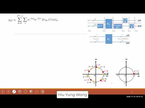
- The algorithm uses 3n qubits: 2n qubits for the Fourier-transform register and n qubits for the function-value register, with 2^n ≥ N.
- Hadamard gates create superposition, and the function is encoded with an exclusive-OR oracle.
- After the quantum Fourier transform, the 2n-qubit register has amplitudes indexed by k from 0 through 2^(2n) − 1.
- The state includes phase factors of the form ω^(−kx), while the function register carries f(x).
- Understanding how the state is built from superposition and the oracle matters more than memorizing the full expression.
- For N = 21, n = 5 because 2^5 = 32 is the smallest power of two at least as large as 21.
- The example therefore uses 15 qubits total: 10 in the Fourier register and 5 in the function register.
- The measured function values follow f(x) = 11^x mod 21, including f(0) = 1 and f(1) = 11.
- The example has period r = 6, so f(x) repeats every six inputs: f(0), f(6), f(12), and f(18) all equal 1.
- Measuring the five-qubit function register collapses it to one function value and leaves input values spaced by the period.
- For an outcome corresponding to f(0), the surviving inputs are represented as x = x₀ + yr, here x = 0 + 6y.
- The next measurement acts on the 2n most significant qubits, collapsing the Fourier index k to a particular measured value k₀.
- The remaining input-register amplitudes retain phase terms that depend on k₀, the offset x₀, and the period r.
- The resulting geometric sum over y determines which k₀ outcomes have substantial measurement probability.
- Each term in the remaining sum contributes a complex phase, so the amplitudes combine through constructive or destructive interference.
- For a strong outcome, increasing y by one must advance the phase by an integer multiple of 2π.
- The Fourier transform uses a 2n-qubit register, so its root of unity has denominator 2^(2n), not 2^n.
- The phase condition leads to r ≈ 2^(2n)d / k₀, or equivalently k₀ / 2^(2n) ≈ d / r for an integer d.
- The measurement reveals k₀, and the register size gives 2^(2n), but the period r and numerator d remain unknown.
- A measured Fourier value therefore supplies a rational approximation to the reciprocal-period relationship, rather than the period directly.
- For illustration, a hypothetical measurement k₀ = 77 with 2^(2n) = 256 gives the ratio 77/256.
- The actual period may not be obvious from that ratio, especially when the registers and candidate periods are large.
- Continued fractions generate candidate denominators for the period, which can then be checked against the modular function.
- Euclid’s algorithm gives the continued fraction 77/256 = [0; 3, 3, 12, 2].
- Its successive convergents include 1/3, 3/10, 37/123, and the exact fraction 77/256.
- The candidate denominators, such as 3, 10, and 123, are tested as possible periods rather than accepted automatically.
- A candidate r must be even, and a^(r/2) must not be congruent to −1 modulo N before the factor-extraction step is useful.
- Compute gcd(a^(r/2) − 1, N) and gcd(a^(r/2) + 1, N); suitable results give nontrivial factors of N.
- If the candidate fails, try another continued-fraction convergent or choose a new random a; the lecture notes that a successful choice occurs with about 50% probability under the stated conditions.
- To learn the derivation, practice reconstructing it rather than only reading an AI-generated solution, which can create a false impression of mastery.
- A general one-qubit state is |ψ⟩ = α|0⟩ + β|1⟩, with complex amplitudes α and β, giving four real parameters before constraints.
- Normalization imposes |α|² + |β|² = 1, reducing the independent real parameters from four to three.
- Writing the amplitudes’ magnitudes as cos(θ/2) and sin(θ/2) packages the normalization constraint into one angle.
- Factoring out a common phase gives the standard form |ψ⟩ = e^(iγ)[cos(θ/2)|0⟩ + e^(iφ)sin(θ/2)|1⟩].
- The common phase γ multiplies the entire state, while φ is a relative phase between the |0⟩ and |1⟩ amplitudes.
- After disregarding the unobservable global phase, θ and φ are the two parameters used to locate a pure qubit state on the Bloch sphere.
- Multiplying a state by e^(iγ) leaves its norm unchanged because e^(−iγ)e^(iγ) = 1.
- Expectation values such as ⟨ψ|M|ψ⟩ are also unchanged: the phase on the bra cancels the phase on the ket.
- The lecture distinguishes a global phase on the whole system from phase differences that can become physically meaningful when they are relative within a larger system.
- The Bloch sphere maps the two parameters θ and φ to a point on a real three-dimensional sphere; it is an embedding, not the qubit’s literal physical space.
- The north pole represents |0⟩, the south pole represents |1⟩, and equal-magnitude superpositions lie on the equator.
- Changing φ while θ = 0 leaves the state at the north pole because the change is only a global phase; every sphere point represents state vectors differing by global phase.
- Antipodal points represent orthogonal states and can serve as the two states of a basis, including the eigenstate pairs of the Pauli operators.
Transcript excerpt
0:07 Last time we talked about Shaw's algorithm and we went all the way to S4 uh C4, right? And now let's just step back look at C3 to see what happened first. After C3, you remember we have uh three N cubits, right? um n needs to be larger than the lumber you want to f I mean two to the power n need to be larger than the lumber you want to factoriize remember but we need free n in order to implement the short algorithm we have uh hard gate what's the purpose not a harder market gate but two nqb hard gate what's the purpose even you don't know algorithm If someone
0:58 asks you what's the purpose of hard market usually >> superposition >> to create superposition right I will give this as a interview question if I interview anyone who want to work in formal computing right this is very basic and then we have the quantum oracle what type of oracle is this we have learned two types or of oracle what type of oracle is this do you know do you remember which are the two types that we have learned exclusive or and >> face. So what what type of oracle is this? Exclusive or oracle. Yeah. So I'm trying to review, right? You you need to understand this for your final exam. So so in other words,
1:47 if I did not teach short algorithm, I give you this circus in principle, you should be able to come up with what I'm saying here. Right? Of course, it's too much for such a short time in final. That's why we won't test that directly. But that is what you are expected to know at this point already. Okay. So, we have this quantum oracle. Usually, we
This is the start of the transcript. Save this video free for the whole transcript, searchable and time-coded.
In this course
Related notes
Summary, takeaways, and chapters were generated by AI from the video's transcript and may contain errors. The video belongs to its creator, Quantum Computing, TCAD, Semicond by Hiu-Yung Wong.