fnb100f261026b
 Watch on YouTube →
Overview
Jeff Hunk explains how natural logarithms solve for time in compound-growth problems, then develops future value of annuities and applies it to a five-year graduate-school savings goal. Using Excel, the class calculates that saving $800 monthly at 6% APR produces about $55,816, compares higher deposits, rates, and timelines, and reviews attendance, grades, and late-work policies.
Key takeaways
- Taking natural logs converts FV/P = (1 + r)^N into a linear equation, so N can be solved as ln(FV/P) divided by ln(1 + r).
- Quarterly compounding produces four periods per year, so a result of 20 quarters must be divided by four to report five years.
- An ordinary annuity pays at each period's end, meaning 60 monthly deposits span 60 months but the first deposit earns interest for only 59 months.
- The future value of an ordinary annuity is payment × ((1 + r)^n - 1) / r, where r is the rate per deposit period, not necessarily the annual rate.
- At $800 per month, 6% APR, and 60 months, the savings plan reaches about $55,816; raising deposits to $860 monthly brings it to roughly $60,000.
- An annuity due earns one extra compounding period per deposit, so its future value equals the ordinary-annuity value multiplied by 1 + the periodic rate.
Chapters
- Jeff Hunk resumes a discussion of Euler's number and natural logarithms as tools for working with exponents.
- A natural logarithm uses e as its base, unlike a common logarithm, which uses 10.
- The class considers why logarithms are useful when the exponent in a compound-growth equation is unknown.
- A logarithm with base 1 cannot distinguish powers because 1 raised to any exponent remains 1.
- Using e as the base lets natural logs handle arbitrary positive real-number values, not just integers.
- The discussion contrasts mentally interpreting a common log of a value such as 13.78 with using a natural log.
- For a power relationship such as Z = X^Y, taking logarithms brings exponent Y down as a multiplier.
- Applying natural logs to FV/P = (1 + r)^N gives ln(FV/P) = N ln(1 + r).
- Solving for N yields ln(FV/P) divided by ln(1 + r), which is the time formula used in the next Excel exercise.
- Students open the Topic 3, Time Value of Money Excel workbook, previously used for single-cash-flow problems.
- The instructor directs students to the course module's reader and Excel file when they cannot find the workbook.
- Jeff Hunk notes that a phone screen is impractical for working in Excel and asks students to identify themselves for attendance.
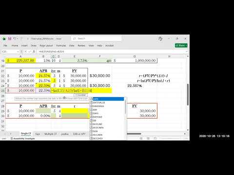
- The example grows $10,000 to $30,000 at approximately 24% annual interest and confirms that it takes five years.
- Excel applies ln(FV/P) divided by ln(1 + APR) to calculate the number of compounding periods.
- The exercise revisits a growth-rate problem previously connected to CAGR, geometric averages, and annualized returns.
- With quarterly compounding, the logarithm formula returns 20 quarters for the same five-year example.
- Because the worksheet labels the result in years, 20 quarters must be divided by four periods per year.
- The conversion returns five years and illustrates why formula output units must match the spreadsheet label.
- The worksheet adds columns for periodic rate and total compounding periods to make formulas easier to read.
- For quarterly compounding, the periodic rate is APR divided by four, and total periods are years multiplied by four.
- The example again produces 20 quarters, then divides by four to report five years.
- A single-cash-flow model has one initial cash outflow and one future cash inflow, such as a bank deposit and its maturity value.
- The same transaction reverses from the bank's perspective: the customer's deposit is the bank's inflow.
- Jeff Hunk introduces multiple cash flows as another way to build future value.
- The example sets a $60,000 graduate-school savings target within five years, based on an estimated $30,000 per year for a two-year program.
- A one-time deposit of roughly $40,000 might grow toward the target, but the example treats that as unrealistic for most students.
- The more practical alternative is a regular monthly deposit from part-time-job income.
- Jeff Hunk defines an annuity as equal payments or deposits made at regular intervals.
- Annuity intervals can be monthly, weekly, quarterly, daily, or annual; the term does not mean payments must be yearly.
- Irregular deposits are excluded from the core model because their timing and amounts are not predictable.
- An ordinary annuity makes each deposit at the end of a period, which fits savings funded by paychecks.
- At $800 per month for five years, there are 60 deposits, but the first deposit compounds for only 59 months.
- The $800 monthly contributions total $48,000 before interest, with later deposits earning progressively less interest.
- A scaled-down example deposits $1,000 at each year-end for five years at 20% interest.
- The first deposit compounds four times, the next three times, then two and one times; the final deposit earns no interest.
- Adding each deposit's accumulated value gives the future value of an ordinary annuity.
- An annuity due begins with a deposit at time zero, so each payment earns one additional compounding period.
- In a five-year example with $5,000 deposits and 10% interest, even the final scheduled deposit earns one period of interest.
- The future value is found by accumulating each deposit and summing the results.
- Compared with an ordinary annuity, an annuity due shifts each payment earlier by one period.
- The difference in future value can be calculated by multiplying the ordinary-annuity result by 1 + the periodic rate.
- This shortcut avoids rebuilding a long series of individual deposit calculations.
- For a monthly savings plan, the first deposit compounds for T - 1 periods, the second for T - 2, and the final deposit for zero periods.
- Each deposit contributes a payment multiplied by a power of 1 + r, where r is the periodic interest rate.
- The repeated terms form a long polynomial, which can be represented compactly using summation notation.
- Summation notation expresses all deposit-growth terms from exponent zero through T - 1 in a compact form.
- The usable ordinary-annuity formula is payment × ((1 + r)^n - 1) / r, with r as the periodic rate and n as the number of periods.
- After introducing the formula, Jeff Hunk pauses for a break before applying it in Excel.
- In the multiple-cash-flow worksheet, the graduate-school example uses an $800 monthly deposit, 6% APR, and a five-year timeline.
- Dividing the 6% APR by 12 gives a 0.5% monthly rate, and five years multiplied by 12 gives 60 deposits.
- The ordinary-annuity formula returns approximately $55,816, which is below the $60,000 target.
- Raising the monthly deposit from $800 to $860 brings the projected balance to about $60,000, slightly above the target.
- An 8% APR still leaves the $800-per-month plan about $1,300 short, illustrating the effect of a higher rate in this example.
- Saving for one additional year creates roughly $9,000 of extra funds, but the class notes that delaying school has an opportunity cost.
- If the first $800 deposit can be made at time zero, the savings plan becomes an annuity due.
- Excel calculates the annuity-due balance by multiplying the ordinary-annuity result by 1 plus the monthly rate.
- Jeff Hunk emphasizes that calculated, highlighted cells should contain formulas rather than manually entered values to avoid inconsistent results.
- The course assignment file combines data across sections and lists attendance, engagement points, Connect chapter-problem averages, and weighted grades.
- Six absences represent about three weeks of a 14-week semester; red-coded absences flag serious attendance concerns.
- The displayed grade is not final because midterm and final scores are not yet included, and weighted averages place more weight on the midterm and final than on the first two quizzes.
- Late chapter work loses 25% per day and receives zero after 20 days; students who stop attending must formally withdraw rather than expecting automatic removal.
Transcript excerpt
1:05 All right. Good afternoon everyone. Good afternoon. Good afternoon. >> Good afternoon, professor. >> Good afternoon. Happy Monday, everyone. Happy Monday. So, let's see who's here. Alrighty. I see Brandon and Luca and Whitmer. Whit and Whitmer Orman and Ty Andre Valentina Olimatu Cortez Haley Aaron Ian. >> Hi. >> All right. All right. Good afternoon everyone. Good afternoon. Happy Monday. All right. So, uh, we are, uh, before we begin, let me, um,
1:55 of course, we're going to pick it up from where we left off last time because last time we were talking about oil's number and how it is, uh, connected with natural law and we were just about to begin um on that. Uh, I mean, we defined oil's number right this way. uh I mean this is my definition this is my interpretation of oilless number and uh uh natural log is the log uh to base e in other words natural log is a log using oiler's number as the base and since uh because since it is diff although although uh we can
2:45 take common log of any number right uh but it's I mean computers can do that easily uh for human brain it's not easy to visualize uh what common log of a number like 13.78 might be right in other words uh what kind of exponent would give you 13.78 based on the you know uh 10 the base of 10. In other words, when you use 10 as the base, the common law, what kind of exponent or the power will give you
3:35 something like 13.78? In other words, some odd numbers, some odd numbers are really really uh difficult to visualize. Right? in terms of common law in terms of right in terms of you know powers of
This is the start of the transcript. Save this video free for the whole transcript, searchable and time-coded.
Related notes
Summary, takeaways, and chapters were generated by AI from the video's transcript and may contain errors. The video belongs to its creator, Jeff Hunk.