fnb100f261001

Overview

Jeff Hunk connects income-statement terms to microeconomics using a hypothetical Dell Model X laptop: direct inputs produce a $300 unit cost, while a $500 assumed price illustrates revenue, variable cost, and cost of goods sold. He then compares revenue and cost curves to explain fixed costs, break-even points, and profit maximization, before distinguishing factory production costs from operating expenses such as rent, clerical salaries, and depreciation.

Key takeaways

In the Dell Model X example, $300 per unit is average variable cost, while total variable cost is $300 multiplied by output; producing 10,000 units therefore yields $3 million in direct costs.
Cost of goods sold and total variable cost describe the same direct production costs under the lesson's simplifying assumption that every unit produced is sold.
A $5 billion plant investment creates fixed costs before production begins, while accounting spreads the plant's cost over its useful life through depreciation.
The gap between total revenue and total cost represents profit; the example's profitable output lies between two break-even points, and the profit maximum need not match the revenue maximum.
Rent and clerical salaries are indirect costs that generally remain stable as output changes, unlike components and assembly-line labor tied directly to production.
When production surges, trained assembly-line workers may require overtime or advance hiring and training, while administrative staffing does not ordinarily need to grow in proportion to output.

Chapters

0:00 Coursework Extensions and Attendance-Roster Questions

Jeff Hunk clarifies that a missed ROI test and the Financial Statements Intro 1 assignment are separate matters.
He extends the Financial Statements Intro 1 deadline to October 4 and explains the stated late penalty of 5% per day.
He asks students to use their correct first and last name so Zoom attendance can be matched to the course roster.

8:20 Why Profitability Makes the Income Statement Important

Jeff Hunk frames profitability as a central consideration when evaluating or investing in a company.
The lesson resumes from the income-statement structure and focuses on the remaining topics of direct and indirect costs.
Direct costs are tied to production inputs, which he describes as capital, labor, and natural resources or raw materials.

14:20 Dell Model X: Identifying Direct Production Inputs

Jeff Hunk uses a hypothetical Dell laptop, the Model X, to illustrate direct production costs.
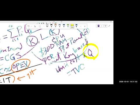
The example identifies factory equipment as capital, assembly-line workers as labor, and components as raw materials.
Laptop inputs include CPU and RAM memory chips, semiconductors, and a flat-panel LED screen, among many other components.

18:18 Calculating Total Variable Cost from a $300 Unit Cost

The hypothetical Model X has a direct production cost of $300 per unit.
Total variable cost equals unit production cost multiplied by quantity produced: at $300 each, 10 units cost $3,000 in total.
The cost varies with output because increasing or decreasing the number of laptops changes total production cost.
Jeff Hunk assumes a perfect demand forecast so quantity produced equals quantity sold, while noting that real inventory can differ.

23:20 Average Variable Cost and Average Revenue

Dividing total variable cost by quantity gives average variable cost, which is also called unit production cost in the example.
Jeff Hunk uses average height as an analogy: sum the measurements, then divide by the number of people.
Dividing sales revenue by quantity gives price, so price is also described as average revenue.

28:55 From Unit Cost to Markup and Cost of Goods Sold

With a $300 unit production cost and an assumed $500 selling price, the difference is initially a markup, not final profit, because indirect costs remain.
Microeconomics calls the aggregate direct cost total variable cost, while accounting calls it cost of goods sold, or COGS.
Under the lesson's assumption that production equals sales, 10,000 laptops at $300 each produce $3 million in COGS.
Revenue and COGS both scale with quantity: revenue uses price times quantity, while COGS uses unit production cost times quantity.

38:00 Plant Investment as a Fixed and Sunk Cost

Fixed cost does not change with production level, unlike the direct costs that rise with each additional unit.
Jeff Hunk estimates that a laptop plant and its equipment could require an initial investment of $5 billion.
That investment is already committed before the first laptop is produced, so the example treats it as a sunk cost and a fixed-cost starting point.

41:30 How Demand Shapes the Model X Revenue Curve

The graph uses quantity on the horizontal axis and dollar amounts, including total revenue and total cost, on the vertical axis.
At an assumed price of $500 per laptop, selling 1,000 units yields $500,000 in revenue.
Revenue can rise as sales expand, then flatten and eventually decline if Dell must lower prices to attract buyers beyond the initial demand.
The example says a lower price, such as $400, may reach another group of buyers, but discounts can reduce total revenue.

47:22 Total Cost, Revenue, and the Profit Gap

Total cost begins at the example's $5 billion fixed investment even when production is zero.
After production starts, the cost curve rises with variable costs, using the $300-per-unit production cost in the laptop example.
Jeff Hunk defines profit as total revenue minus total cost and represents it as the vertical distance between the two curves.
A student question about adding product lines prompts the clarification that a company could introduce a new model, while the graph initially isolates one product.

52:10 Two Break-Even Points and the Profit-Maximizing Output

Where total revenue and total cost intersect, profit is zero; the graph shows a first and a second break-even point.
Production between those intersections is profitable in the illustrated model, while output below the first or beyond the second produces a loss.
The output that maximizes the gap between revenue and cost is the profit-maximizing level.
The revenue-maximizing output is not necessarily the profit-maximizing output, which Jeff Hunk places slightly earlier in the example.

59:25 Break-Even Graphs as an Income-Statement Interpretation

Jeff Hunk connects the graph to income statements by showing that profit or loss changes with output level.
A simplified break-even chart may use straight lines around the first break-even point.
Extending the model beyond that local approximation produces curved revenue and cost patterns rather than indefinitely straight lines.
The graph omits interest and taxes, so it illustrates the broad profit relationship rather than every income-statement line.

1:02:00 Coffee-Shop Rent as a Fixed Operating Expense

A campus coffee shop illustrates rent as a fixed cost because the monthly payment does not rise or fall with sales.
At $5 per cup, monthly revenue of $50,000 corresponds to 10,000 cups sold.
If each cup costs $2 to make, 10,000 cups generate $20,000 in variable costs, leaving $30,000 before rent and other expenses.
The example uses monthly rent of $5,000 and contrasts normal, stronger, and weaker sales months to show that rent stays constant.

1:06:15 Production Workers Versus Clerical Staff

When laptop orders double from 10,000 to 20,000 units in a quarter, direct inputs such as components and production labor must increase if capacity allows.
Assembly-line roles require trained workers, so staffing cannot always be doubled immediately; overtime can cover a short-term surge while new workers are trained.
Secretaries and other clerical staff are indirect to production, so their headcount and hours do not normally need to double with output.
Jeff Hunk uses this contrast to explain why some labor costs vary with production while administrative payroll behaves more like a fixed expense.

1:12:30 Operating Expenses, Depreciation, and Accounting Treatment

Rent, fixed administrative salaries, and general administrative costs are examples of operating expenses, or OPEX.
Accounting recognizes plant investment through depreciation rather than treating the entire purchase as a single period expense.
The $5 billion plant investment is spread across its useful life; Jeff Hunk gives 10 to 15 years as a typical illustrative range.
He contrasts microeconomics' treatment of initial investment as a fixed-cost chunk with accounting's practice of allocating asset cost over time.

1:15:35 KLR Recap and Class Wrap-Up

In the closing question, Jeff Hunk defines KLR as capital, labor, and raw material or natural resources.
He links KLR to variable cost because these are direct inputs used in production.
The class ends with a reminder to see the students the following Tuesday.

Transcript excerpt

1:08 All right. Good afternoon everyone. Good afternoon. >> Good afternoon. >> Happy good afternoon. Happy Thursday. >> Afternoon. >> All righty. Alrighty. I see uh how many people are here? Uh looks like I'm seeing at least nine people, right? just nine people. Well, something this is this is so unexpected and okay. Um All right. Where was I? I think I somebody Yeah, there was a uh

2:05 chat pop up in the chat. >> Yeah, Collins. Um uh you're asking if it is possible I can reopen the first ROI videos. Um uh actually uh uh no um instead I've been telling you uh in the uh if you go to the announcements right I've given you my YouTube channel name. Yeah, I have I know your YouTube channel, but you still I still can't access the test if I don't click on that um ROI. So >> Oh, okay. So, uh but you don't have ROI.

2:58 Oh, ROI 2. No, you don't have any ROI. I mean, your your ROI test one and two are all done by uh last Sunday. Yeah. So for the next test, u the one I missed, the first one I didn't click, will that affect it? >> Uh >> if you missed I mean listen, if you missed uh any test >> uh I mean uh basically you need to do it within the uh within the uh the assigned window. Um and uh ROI I don't know which one you missed but you know if you missed ROI

3:48 too it's been already a week and there is always late penalty. I mean if you make up there's you know a late penalty of 5% per day late. If you're a week late that's already 35% right penalty uh minus 35%. If you are two weeks late then you know

This is the start of the transcript. Save this video free for the whole transcript, searchable and time-coded.

Related notes

Summary, takeaways, and chapters were generated by AI from the video's transcript and may contain errors. The video belongs to its creator, Jeff Hunk.