ES.1802, October 1, 2026

Overview

The lecture derives the tangent plane for an explicit surface z=f(x,y), then uses a custom VR calculus app to explore tangent planes and level curves on functions including a saddle and paraboloid. It develops local linear approximation as the function value plus the gradient dotted with a small coordinate change, explains sensitivity through partial derivatives, and introduces Jacobian matrices as the tool for organizing multivariable chain rule calculations.

Key takeaways

For z=f(x,y), the tangent plane at (x₀,y₀) is the local linear model f(x₀,y₀)+f_x(x₀,y₀)(x−x₀)+f_y(x₀,y₀)(y−y₀).
The normal vector to the tangent plane of an explicit surface z=f(x,y) can be derived by crossing slice tangent vectors, giving (f_x,f_y,−1).
A variable's local sensitivity is determined by the absolute value of its partial derivative, so the largest-magnitude partial identifies the strongest input influence near a point.
The multivariable linear approximation generalizes to any number of inputs as f(x)≈f(x₀)+∇f(x₀)·(x−x₀).
For a vector-valued function F=(u,v) of (x,y), the Jacobian has rows ∇u and ∇v, arranging all component-by-input partial derivatives in one matrix.
When f depends on x and y and both depend on t, the multivariable chain rule adds the two paths: df/dt=f_x·dx/dt+f_y·dy/dt.

Chapters

0:00 Deriving the Tangent Plane from Two Surface Slices

For an explicit surface z=f(x,y), slicing at constant y and constant x produces two curves through the point of tangency.
The slice tangent directions are represented by vectors (1,0,f_x) and (0,1,f_y), using the corresponding partial derivatives at the point.
Their cross product gives a normal vector (f_x,f_y,-1), which combines with the point of tangency to define the plane.
The derivation applies directly to explicit surfaces z=f(x,y); implicit surfaces such as x²+y²+z²=5 require a different setup.

6:43 Exploring Tangent Planes and Level Curves in a VR Calculus App

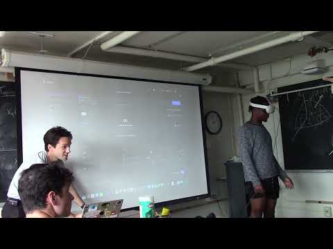
Students use VR headsets and hand-tracked controls to select functions, adjust the tangent point with sliders, and rotate the plotted surface.
The app displays tangent planes and level curves, including the saddle-shaped level curves reviewed from an earlier class.
Users can lower the surface opacity, reposition the axes, and inspect the level curves from near the surface plane.
The custom app loads plots faster than an earlier version that had noticeable delays, making it practical for in-class exploration.

15:03 Using the Tangent Plane as a Local Model

A tangent line approximates a single-variable function near its point of tangency; the analogous local model for a surface is its tangent plane.
The plane approximates the surface only near the selected point, with larger discrepancies as the input moves farther away.
The VR paraboloid demonstration makes the local fit visible by showing the tangent plane and surface together.
The class uses this geometric idea to motivate tangent plane approximation before moving to multivariable chain rule.

18:43 From the Single-Variable Tangent Line to Linear Approximation

For y=f(x), a small input change Δx produces an approximate output change Δy=f'(x₀)Δx at the point x₀.
Rearranging gives the tangent-line estimate f(x)≈f(x₀)+f'(x₀)(x−x₀).
At x=x₀, the change term vanishes, so the approximation returns the known value f(x₀).
The equation is useful when a nearby function value is easier to estimate from the tangent line than to calculate directly.

23:23 Building the Two-Variable Tangent Plane Approximation

For z=f(x,y), changes in both x and y contribute to changes in z through f_x and f_y.
Near (x₀,y₀), the approximation is f(x,y)≈f(x₀,y₀)+f_x(x₀,y₀)(x−x₀)+f_y(x₀,y₀)(y−y₀).
Each partial-derivative term accounts for one variable's contribution to the local change in the function.
The approximation is linear even when the original function is nonlinear, which can simplify calculations such as small-angle estimates.

30:01 Sensitivity and the Gradient-Dot-Displacement Form

Sensitivity to a variable is measured by the magnitude of its partial derivative; the larger absolute partial indicates the stronger local effect.
For a function of x, y, z, a, and b, the same approximation pattern adds one partial-derivative term for each input variable.
The collection of partial derivatives is the gradient, and the input changes form a displacement vector.
The general local model is f(x)≈f(x₀)+∇f(x₀)·(x−x₀), extending the approximation to any number of input variables.

33:46 Scalar-Valued Functions, Vector-Valued Functions, and Gradients

A scalar-valued function such as f(x,y) returns a number for each input pair.
The gradient of f is a vector-valued function: it returns the vector of partial derivatives, here (f_x,f_y).
The lecture introduces compact notation such as f_x and f_y for partial derivatives with respect to x and y.
A general vector-valued function can map each input pair to a vector, for example (u(x,y),v(x,y)).

37:48 Constructing the Jacobian Matrix from Component Gradients

For F(x,y)=(u(x,y),v(x,y)), the Jacobian is a 2-by-2 matrix containing the derivatives of both output components.
Its rows are the component gradients: [u_x,u_y] and [v_x,v_y].
The same matrix can be denoted ∂(u,v)/∂(x,y), making the input and output variables explicit.
The Jacobian generalizes the gradient's derivative information to vector-valued functions and prepares for matrix-based chain rule calculations.

42:53 Multivariable Chain Rule and the Jacobian Product Preview

If f depends on x and y, and both x and y depend on t and s, then t influences f through two paths.
The derivative with respect to t is f_x·x_t + f_y·y_t, adding the contributions through x and y rather than treating them as one path.
The factors in each path do not simply cancel to produce a single derivative, because f depends on t indirectly through multiple variables.
The next class will organize all such derivatives by multiplying the Jacobian from f to (x,y) by the Jacobian from (x,y) to (t,s).

Summary, takeaways, and chapters were generated by AI from the video's transcript and may contain errors. The video belongs to its creator, ChristianAltoSax.