EM fields lecture 29 - Boundary condition for vector fields between media & 3D to 1+2D space
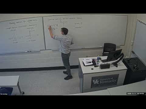
Overview
Tim Gorringe derives general boundary conditions for a vector field by applying the divergence theorem and Stokes' theorem to small surfaces that cross an interface. The derivation separates the field jump into a normal component controlled by flux sources and tangential components controlled by circulation sources, framing the interface as one normal dimension plus a two-dimensional surface.
Key takeaways
- A boundary condition for the normal component follows from the divergence theorem: the jump in the normal field is determined by the flux source integrated through a thin pillbox crossing the interface.
- A boundary condition for tangential components follows from Stokes' theorem: circulation around a narrow loop crossing the interface relates the tangential field jump to the curl source.
- An interface can be treated as a one-plus-two-dimensional space: one normal direction and a two-dimensional tangent plane.
- At a conductor-vacuum boundary in electrostatic equilibrium, the field inside the conductor is zero, the exterior tangential field is zero, and the exterior normal field is set by surface charge density divided by ε₀.
- A finite field jump in the zero-thickness interface limit is associated with a source concentrated at the boundary; without the relevant flux or circulation source, the corresponding field component is continuous.
Chapters
- Electromagnetic problems often place fields across interfaces such as conductor-vacuum or dielectric-vacuum boundaries.
- The normal component is perpendicular to the interface; the tangential component lies in its plane.
- Field divergence and curl determine whether these components remain continuous or change across the boundary.
- Electromagnetic boundary conditions determine the reflected and transmitted portions of light at an air-glass interface.
- The transmitted ray follows the law of refraction, while the reflected ray follows the law of reflection.
- The lecture idealizes a real material interface, which has finite thickness across many atoms or molecules, as an infinitely thin transition.
- The boundary description decomposes three-dimensional space into one direction normal to the interface and two directions tangent to it.
- For a conductor-vacuum boundary, the conductor is medium 1 and vacuum is medium 2.
- In electrostatic equilibrium, the electric field inside the conductor is zero, and the field just outside has no tangential component.
- Tim Gorringe represents a general vector field as A and its scalar flux source as B, with divergence of A equal to B.
- A unit normal vector n identifies the direction perpendicular to the interface and selects the normal field component.
- A thin pillbox Gaussian surface straddling the boundary captures flux through a top cap, a bottom cap, and a sidewall.
- The pillbox end caps have area a, while its small height is h; the top cap lies in medium 2 and the bottom cap in medium 1.
- As h approaches zero, the sidewall contribution vanishes, leaving the difference between the two end-cap fluxes.
- The divergence theorem equates that flux difference with the integral of B over the pillbox volume, giving a normal jump controlled by the source integrated across the interface.
- The second boundary relation uses a vector source C for the curl of A, because curl is itself a vector.
- Stokes' theorem equates circulation around a closed loop with the surface integral of C through the loop.
- A narrow rectangular loop crossing the interface isolates the tangential components of A in media 1 and 2.
- The loop has length L along the interface and a small height h across it.
- As h approaches zero, circulation along the two short vertical edges vanishes, leaving the top and bottom tangential field contributions.
- The loop's surface area is Lh, so the curl source contributes through its component normal to the loop surface.
- The derivation defines n as the interface normal, n-prime as the loop-surface normal, and t as a tangent direction formed from their cross product.
- Dot and cross product identities reorganize the circulation equation so it directly relates the tangential field difference to the curl source.
- The resulting tangential jump is a two-dimensional vector on the interface, distinct from the scalar normal jump.
- The normal component of A is selected by dotting its change across the boundary with n, and its jump is governed by the flux source B.
- The tangential component is selected using a cross product with n, and its jump is governed by the circulation source C.
- A zero source of flux or circulation implies no corresponding normal or tangential jump, respectively.
- The abstract boundary relations apply to any vector field A, with B representing its flux source and C its circulation source.
- For the conductor-vacuum example, the exterior normal electric field depends on surface charge density as σ/ε₀, while the tangential field at the surface is zero.
- The next class is set to make the general relations concrete for electrostatic fields and material boundaries.
Transcript excerpt
0:02 Many problems in electrostatics actually many problems in electromagnetism involve um fields in regions where there's different material materials or different media and there's boundaries between these materials or the media. So an example uh that we've met is a boundary between a region of conductor and vacuum and a an example that we will meet is a boundary between um a dialectric insulator and and vacuum. And today's class and Friday's class are about uh conditions what we call boundary
0:51 conditions that we can impose on the the fields the vector fields the electrical fields say u at the um interfaces or the the uh boundaries between two media. Um just like uh fields like electric fields are determined by their divergence and curl properties. So their divergence and curl properties determine um the the nature of the fields. Um the boundary conditions imposed on fields they're also determined by the divergence and curl properties of the field. So they
1:38 dictate the boundary conditions. Um what our task is today, what our job is today is really to map the field properties. We're going to just talk about an arbitrary field, but map field properties. So that will be what is the divergence of the field? Uh what is the curl of the field? map those onto a interface or a boundary between two media. And the key idea in doing that is that um we're going to think about the field at the me at the interface at the boundary between two media say between conductor and vacuum or insulator and vacuum as um
2:28 having two distinct components. One is the field component that's normal right angles to the interface between the two media and then the other one is the field component that's um tangent in the plane of the interface between the
This is the start of the transcript. Save this video free for the whole transcript, searchable and time-coded.
In this course
Related notes
Summary, takeaways, and chapters were generated by AI from the video's transcript and may contain errors. The video belongs to its creator, tim gorringe.