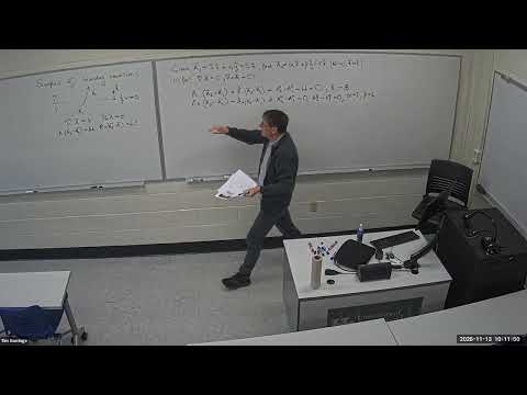
EM fields lecture 30 - example of boundary condition for general fields and electrostatic fields
Overview
The lecture derives boundary conditions for a general vector field, then applies them to electrostatics: the normal field jump is set by surface charge, while the tangential component is continuous because the electrostatic field has zero curl. Examples check these rules for a charged sheet and parallel-plate capacitor, then use the induced surface charge on a conducting sphere to determine the field just outside it.
Key takeaways
- For the general vector-field boundary conditions used in the lecture, divergence or flux sources determine the normal-component jump, while curl or circulation sources determine the tangential-component jump.
- In the electrostatic examples with permittivity ε₀, a surface charge density σ produces a normal electric-field jump of σ/ε₀, while the tangential component is continuous.
- An infinite charged sheet has fields of magnitude σ/(2ε₀) on its two sides; because the directions are opposite, the normal-field difference across the sheet is σ/ε₀.
- An ideal parallel-plate capacitor has field magnitude σ/ε₀ between its plates and zero outside, so crossing a plate gives the same normal-field jump as crossing a charged sheet.
- For the conducting sphere's induced distribution σ_s = −σ₀ cos θ, the field immediately outside points inward at the north pole, outward at the south pole, and vanishes at the equator.
- The zero field inside a conductor and continuity of the electrostatic tangential field require the field at its surface to be normal to the surface.
Chapters
- The interface separates regions 1 and 2, with its unit normal defining perpendicular and tangential directions.
- The jump in the normal component is related to the field's divergence or flux source.
- The jump in the tangential component is related to the field's curl or circulation source.
- The derivation takes the boundary thickness h to zero.
- A general field A is specified on one side of a boundary in the plane z = constant, whose normal is the z direction.
- With zero flux and zero circulation sources, the normal and tangential boundary conditions require all three field components to match.
- For the example's initial components 3, 4, and 5, the field on the other side remains unchanged.
- The example assigns a flux contribution hB = 2 and a tangential circulation contribution hC = 3 in the x direction.
- The normal component changes by 2, taking the initial z component from 5 to 7.
- Applying the cross-product direction of the circulation condition gives the corrected tangential components: x remains 3 and y changes from 4 to 7.
- The worked result illustrates that flux controls the normal jump, while circulation controls the tangential jump.
- For the electrostatic field, charge density is the flux source, with volume charge density contributing as ρ/ε.
- The lecture models a thin boundary region of thickness h and area A containing charge Q, so its volume is Ah.
- Taking h to zero converts the volume charge description into surface charge density and gives a normal-field jump of σ/ε in the setting considered.
- Because the electrostatic field has zero curl, its tangential component is continuous across the boundary.
- A positively charged infinite sheet produces fields of magnitude σ/(2ε₀) on each side, directed away from the sheet.
- With region 2 above and region 1 below, the normal field changes from −σ/(2ε₀) to +σ/(2ε₀).
- The resulting jump is σ/ε₀, matching the surface-charge boundary condition.
- Both sides have zero field component parallel to the sheet, consistent with tangential-field continuity.
- Oppositely charged parallel sheets create a uniform field of magnitude σ/ε₀ between the plates and zero field outside.
- At the upper plate, the normal field changes from zero in the exterior region to σ/ε₀ between the plates.
- The field has no component parallel to the plates, so its tangential component remains zero across the interface.
- The capacitor provides a second direct check of both electrostatic boundary conditions.
- A conducting sphere inserted between capacitor plates has zero electric field inside the conductor.
- Induced negative and positive charges on opposite sides of the sphere exclude the applied field from its interior.
- Far from the sphere, the field remains approximately the original uniform capacitor field; near the surface, field lines meet the conductor perpendicularly.
- Unlike a conducting slab's approximately uniform face charges, the sphere's induced surface charge varies with position.
- The sphere's surface charge density is specified as σ_s = −σ₀ cos θ, with θ measured from the vertical axis.
- At the north pole, θ = 0 and the induced charge density is −σ₀; at the south pole, θ = 180° and it is +σ₀.
- At the equator, θ = 90° and the charge density vanishes.
- The charge distribution supplies the local input needed to apply the normal-field boundary condition around the sphere.
- Since the field inside the conductor is zero, the outside normal field is set by the local surface charge density divided by ε₀.
- At the north pole, the field points toward the sphere's center with magnitude σ₀/ε₀.
- At the south pole, the field points radially outward with magnitude σ₀/ε₀.
- At the equator, zero surface charge gives zero field immediately outside; intermediate latitudes have intermediate field strengths.
- The lecture's examples progress from a general vector field to a charged sheet, a parallel-plate capacitor, and a conducting sphere.
- Across each electrostatic boundary, surface charge determines the jump in the normal field component.
- The tangential field remains continuous because the electrostatic field has zero curl.
Transcript excerpt
0:02 Last class we talked about boundary conditions at the interface between two different media. We talked them about them for a general vector field. Uh our application will be the electrostatic field. Um today's class I I'll just start by writing down a couple of equations to remind us of last class. Then I just want to work through some examples of boundary conditions. Uh the first one I have is for some arbitrary vector field and how that changes at a boundary um when there is or isn't sources of circulation and flux at that field. And then the uh later ones are boundary conditions for the electrostatic field at a familiar
0:52 situation. So when you have sheets of charge um or planes of charge when you have um spherical distributions of charge or spherical shells of charge we look at the boundary condition there um and also talk say a few words about u the u changing of the direction of the electrical field of the boundary which is essentially a refraction of the electrostatic field of the boundary. Okay. So, just as a quick reminder because we're going to keep using it, we talked about a boundary between two different media in the last class. Here are the two media separated by some horizontal line and some unit vector characterizing the boundary. And um in general we imagined
1:44 a vector field in the lower region one a vector field in the lower re upper region two and how they're related and we discovered the change in the vector field a across the boundary between the two regions. It was related to the field properties of the vector field. um that is the um the divergence and the the curl of the vector field. uh and um the sources of
This is the start of the transcript. Save this video free for the whole transcript, searchable and time-coded.
In this course
Related notes
Summary, takeaways, and chapters were generated by AI from the video's transcript and may contain errors. The video belongs to its creator, tim gorringe.