EM fields - test two review
Overview
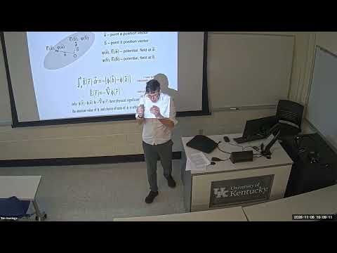
Tim Gorringe reviews the electrostatics material for test two, moving from the curl-free electric field and scalar potential through conductors, capacitance, and stored energy. He connects these topics with worked examples including a uniformly charged spherical shell, a spherical capacitor, a four-ion crystal, and far-field multipole expansions used to find interaction energies, forces, and torques.
Key takeaways
- Because an electrostatic field is curl-free, it can be represented as E = -∇φ; potential differences, rather than absolute potential values, determine physical effects.
- A uniformly charged spherical shell produces the same potential and field as a point charge outside it, but has constant potential and zero electric field inside.
- At electrostatic equilibrium, a conductor has zero internal field and is an equipotential; its exterior normal field is set by surface charge density through E⊥ = σ/ε₀.
- Capacitance is the ratio Q/ΔV and depends on conductor geometry, while potential coefficients encode the geometry-dependent relationship between multiple conductor charges and potentials.
- Electrostatic energy can be calculated through assembly work, charge-potential sums, or field energy; the factor of one half in charge-potential expressions prevents counting each pair interaction twice.
- For a localized distribution at large distances, the lowest-order nonzero multipole moment controls the potential, while multipole interaction terms also provide the system's energy, force, and torque.
Chapters
- Test one covered electrostatic forces and fields; test two focuses on electrical potential and energy.
- The review covers potentials from point charges and continuous charge distributions, conductor properties, and capacitors.
- The final topics are electrical energy and multipole expansions for describing charge distributions at large distances.
- The electrostatic line integral from point A to point B is path-independent, so the integral around a closed loop is zero.
- A curl-free electric field can be written as the negative gradient of a scalar potential: E = -∇φ.
- Only potential differences are physically significant, so the zero of potential can be chosen wherever convenient.
- The line integral obeys ∫A→B E·dl = φ(A) - φ(B), linking field calculations to potential differences.
- The shell's potential is found by summing point-charge contributions from surface elements dQ = σ dA.
- On a sphere, the surface element is constructed from polar and azimuthal angle increments, dθ and dφ.
- The integral yields two cases: outside the shell, the potential is that of a point charge with the shell's total charge.
- Inside the shell, the potential is constant and depends on the shell's charge and radius, rather than on the field-point radius.
- For the spherically symmetric shell, φ depends only on r, so only the radial term of the spherical-coordinate gradient contributes.
- Outside the shell, differentiating the 1/r potential gives an electric field proportional to 1/r², identical to a point charge's field.
- Inside the shell, the constant potential has zero gradient, so the electric field is zero.
- When an external field is applied, free charges move briefly and redistribute until electrostatic equilibrium is reached.
- The electric field inside a conductor is zero, and the field component parallel to its surface is also zero.
- A conductor has zero volume charge density in equilibrium, although charge can reside on its surface.
- The conductor is an equipotential, and its surface charge density is related to the perpendicular field by E⊥ = σ/ε₀.
- Before inserting the slab, oppositely charged plates produce a uniform field σ/ε₀ between them; the fields cancel outside the plates.
- Free charges in the slab redistribute to make the field inside the conductor zero and its volume charge density zero.
- Negative surface charge forms on the slab face toward the positive plate, while positive surface charge forms on the face toward the negative plate.
- The induced surface charges redirect the field so that it remains perpendicular to the conductor's surfaces and absent from its interior.
- Potential coefficients relate each conductor's potential to the charges on all conductors in the arrangement.
- For two conductors, the coefficients form a 2 by 2 matrix; three conductors require a 3 by 3 matrix.
- The coefficients depend on conductor geometry and spacing, not on the chosen charges or potentials.
- The coefficient matrix is symmetric in its off-diagonal terms, reducing the number of independent values.
- A spherical capacitor consists of an inner conducting sphere and an outer conducting shell carrying equal and opposite charges.
- The potential difference is calculated by integrating the inverse-square electric field through the gap between the conductors.
- Capacitance is the stored charge divided by the potential difference, so the charge cancels and the result depends on geometry.
- The same capacitance can be derived from the potential-coefficient equations by setting the conductor charges to Q and -Q.
- Energy can be calculated as the work required to assemble a charge distribution, by summing charge interactions, or from charge in the potential of other charges.
- For a four-ion crystal example, nearest-neighbor and opposite-pair interactions provide a check against the assembly-work method.
- For continuous charge, the potential-energy expression integrates charge in the potential created by the other charge, with a factor of one half to avoid double-counting.
- The field description stores energy in the electric field, with energy density proportional to ε₀E².
- For a localized charge distribution viewed from far away, the potential can be expanded in monopole, dipole, quadrupole, and higher moments.
- The first nonzero moment dominates at large distance: monopole terms scale as 1/r, dipole terms as 1/r², and higher terms decay faster.
- Moments are calculated by summing over point charges or integrating over charge elements; a spherical surface with charge density proportional to cos θ provides a dipole example.
- Multipole interaction formulas give energy, force, and torque for a charge system such as a dipole in an external point-charge, uniform, or dipole field.
Transcript excerpt
0:01 So today's class I just wanted to run through a number of slides to cover the materials since test one and this is going to be on test two. Big picture test one really covered forces and fields in electrostatics and test two is covering energy and potential in electrostatics. And then after test two we're going to be talking about materials, matter and we're going to be talking about some special methods, mathematical methods. So that's how the course was laid out. That's how the course was constructed. This is the material for test two. We
0:52 started with some remarks about the electrostatic field that it was a curbless field. That led us to introduce the concept of the electrical potential, a scalar potential, and we solve problems of the scalar potential of various arrangements of charge, assemblies of point charge distributions, continuous distributions of charge. We talked about the particular properties, characteristics of electrical conductors. So we spent some time on the nature of the potential on the surface and the volume of electrical conductors and we
1:41 looked at some problems involving electrical conductors that can include capacitors. We then moved on after the full break to discuss the electrical energy of arrangements of charge or arrangements of conductors. it could be point charges, could be continuous distributions of charges, say could be charges distributed on conductors. Um we discovered there's various ways of describing the electrical energy of a a charge distribution. You could figure out the electrical energy by simply assembling the charge distribution and totaling up how many joules of work you had to do to assemble the charge
2:28 distribution. Um that's a very sort of physical, natural way of thinking about the energy stored in a charge distribution. Typically it's a um a painful way to calculate the energy
This is the start of the transcript. Save this video free for the whole transcript, searchable and time-coded.
In this course
Related notes
Summary, takeaways, and chapters were generated by AI from the video's transcript and may contain errors. The video belongs to its creator, tim gorringe.