Electromagnetic fields, lecture 4- - quadrupole field, div / grad, line / surface ints, & potentials
Overview
Tim Gorringe uses the quadrupole field A = (y, x, 0) to demonstrate vector calculus in Cartesian coordinates, including field sketches, a closed-loop circulation integral, cube-face flux integrals, curl, and divergence. The field has zero curl and zero divergence everywhere, so it can be written both as the gradient of the scalar potential xy and as the curl of a vector potential with z-component (y² − x²)/2; Gorringe also explains the identities curl(grad U) = 0 and div(curl A) = 0.
Key takeaways
- For A = (y, x, 0), div A = 0 because ∂y/∂x and ∂x/∂y are both zero.
- The same field is curl-free because its z-component of curl is ∂x/∂x − ∂y/∂y = 1 − 1 = 0.
- A square loop with side length 1 in the xy-plane has zero net circulation: its nonzero side contributions are +1 and −1.
- A unit cube has zero net flux for this field: the front and back faces contribute zero, and opposite side-face fluxes cancel in pairs.
- The scalar potential U = xy generates the quadrupole field through ∇U = (y, x, 0).
- The vector potential A = (0, 0, (y² − x²)/2) generates the same field through ∇ × A, illustrating the divergence-free field representation.
Chapters
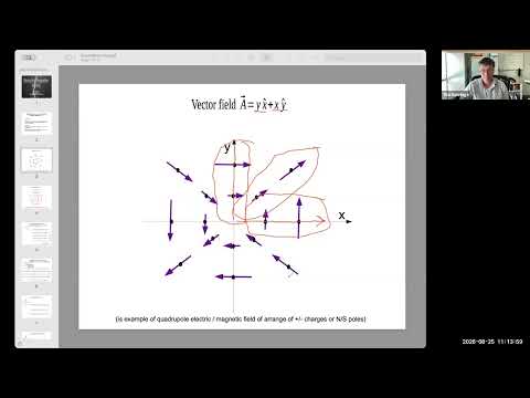
- Gorringe introduces A with x-component y, y-component x, and no z-component.
- The field models the local pattern near an electric quadrupole or a magnetic quadrupole.
- The lecture applies line and surface integrals, curl, and divergence to this one field.
- On the x-axis, y = 0, so the field points in the y-direction with magnitude proportional to x.
- On the y-axis, x = 0, so the field points in the x-direction with magnitude proportional to y.
- At the origin, both coordinates vanish and the field is zero.
- Combining the x- and y-components produces curved field lines that sweep around the origin in four regions.
- The field direction reverses across the x- and y-axes, while its magnitude increases away from the origin.
- A charge arrangement with positive charges on opposite square corners and negative charges on the other corners creates the described electrostatic pattern.
- Gorringe chooses a closed square in the xy-plane with corners at (0,0), (1,0), (1,1), and (0,1).
- The circulation integral adds the component of A parallel to each directed line element ds.
- He splits the loop into four sides, tracking whether x or y increases or decreases along each path.
- The first side lies at y = 0, making its x-directed contribution zero.
- The vertical side at x = 1 contributes 1, while the top side, traversed from x = 1 to 0, contributes −1.
- The final side lies at x = 0 and contributes zero, so the total circulation around the square is zero.
- The closed surface is a cube extending one unit along x, y, and z from the origin.
- Gorringe divides the total flux integral into contributions from the cube’s six faces.
- The outward area vectors point along positive or negative coordinate axes, depending on the face.
- The front and back faces have zero flux because A has no z-component.
- Integrating the x-component over the left and right faces gives fluxes of −1/2 and +1/2.
- The upper and lower faces likewise contribute opposite fluxes, so the net flux through the cube is zero.
- The square’s zero circulation and the cube’s zero net flux result from cancellations among individual path segments and faces.
- Curl describes the local source of circulation, while divergence describes the local source of flux.
- The next calculations test whether the observed cancellations hold throughout space, not just for the chosen square and cube.
- Gorringe writes the Cartesian curl using the determinant form of ∇ × A.
- The x- and y-components vanish because the field has no z-dependence or z-component.
- The z-component is ∂Ay/∂x − ∂Ax/∂y = 1 − 1 = 0, so the field is curl-free everywhere.
- In Cartesian coordinates, div A is ∂Ax/∂x + ∂Ay/∂y + ∂Az/∂z.
- For Ax = y and Ay = x, both relevant derivatives are zero, and Az is identically zero.
- The resulting zero divergence means the field has no local sources or sinks of net flux.
- Gorringe clarifies the correct correspondences: a curl-free field can be represented as the gradient of a scalar potential.
- A divergence-free field can be represented as the curl of a vector potential.
- The quadrupole field satisfies both conditions, so it admits both kinds of potential representation.
- The identity ∇ × ∇U = 0 follows because mixed second partial derivatives cancel in pairs.
- Geometrically, ∇U points in the same direction as the differential operator ∇, so their cross product vanishes.
- For this field, U = xy gives ∇U = (∂U/∂x, ∂U/∂y, 0) = (y, x, 0).
- The identity ∇ · (∇ × A) = 0 follows because paired mixed second derivatives cancel.
- A vector potential for the quadrupole field is A = (0, 0, (y² − x²)/2); taking its curl returns (y, x, 0).
- The scalar- and vector-potential identities provide tools for representing electric fields and magnetic fields in later electromagnetism.
Transcript excerpt
0:02 In the last classes, we've been introducing a mathematical language of vector calculus, differential vector calculus, integral vector calculus for describing vector fields and also describing scalar fields. Uh we talked about div, curl and grad in vector calculus. uh differential vector calculus. We talked about line surface integrals uh for integral vector calculus. Uh these quantities help us describe uh field properties, vector field properties like the flow of the field, like the rotation of the field, scalar field properties like the slope
0:50 of the uh the the scalar field. In today's class, I want to apply um these methods uh provide an example of these methods for a particular field. We've been working in cartesian coordinates, rectangular coordinates um where we're working with um x y and z coordinates, axes and unit vectors. uh we're going to work on a particular field that's expressed in rectangular coordinates and that field is upstairs here. Uh I'm going to call that field A. The vector field A is has an x component and it has a y component. Um
1:40 the x component depends on the y-coordinate. Interestingly, um the y component depends on the xcoordinate. Interestingly, it doesn't have a z component. This is actually a famous field, a famous vector field. Uh this field appears in electrostatics. It appears in magnetostatics. Um it's the field of a electric quadripole. what we call an electric quadripole or a magnetic quadripole. Um you can make an electrical quadripole with um two positive charges and two negative charges. If you arrange the positive charges on opposite corners of a square, the negative charges on the
2:28 other opposite corners of a square, that creates an electrostatic quadripole. And in the region of the center of that square, you would get a field that would
This is the start of the transcript. Save this video free for the whole transcript, searchable and time-coded.
In this course
Related notes
Summary, takeaways, and chapters were generated by AI from the video's transcript and may contain errors. The video belongs to its creator, tim gorringe.