EECS 373 - Fall 2026 - Lecture 13: "Overview: Analog Signals"
Overview
The lecture explains how embedded systems bridge analog phenomena and digital computation with analog-to-digital converters (ADCs), digital-to-analog converters (DACs), sampling, and quantization. It develops practical design rules around the Nyquist-Shannon theorem, aliasing, ADC resolution and reference ranges, then applies them to sensor conversion, resistance and current measurement, and an EMI-sensing wristband example.
Key takeaways
- To reconstruct a signal without aliasing, sample at least twice its highest frequency; practical instruments often oversample, and the lecture gives five samples per cycle as a useful oscilloscope rule of thumb.
- ADC resolution depends on both bit depth and reference range: increasing the bit count or narrowing the range around a safely contained signal reduces voltage per code.
- For a 12-bit ADC over 0 to 3 V, the lecture's maximum quantization error is about 0.36 mV, which can be smaller than noise from the analog front end.
- Sensor software must combine two mappings: convert ADC counts to voltage using the ADC reference range, then convert voltage to units such as temperature using the sensor datasheet.
- An ADC measures voltage directly, but a voltage divider can reveal an unknown resistance and a precise shunt resistor can convert current into a measurable voltage drop.
- A Cortex-M4 wristband can use an ADC to capture device-specific EMI signatures through the body, then use filtering and machine learning to identify touched objects.
Chapters
- Sensors such as microphones, temperature sensors, and light sensors produce analog signals, commonly represented as voltages, that an embedded system must measure.
- An ADC converts an analog voltage into a digital value; a microphone signal can be digitized for recording as an MP3.
- A DAC converts digital data into voltage for outputs such as speakers and radio transmitters.
- A speaker's voice coil moves a diaphragm when voltage passes through it, turning the DAC's output into sound.
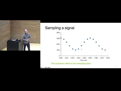
- Sampling rate is how often an ADC measures a changing analog signal, expressed in samples per second.
- The lecture uses audio specifications of 24-bit resolution and 44.1 kHz sampling as an example.
- Human hearing reaches roughly 20 kHz, so audio sampling must exceed 40 kHz to capture that range, with additional headroom for filtering.
- Telephone voice has often used an 8 kHz sampling rate because most speech information lies below about 4 kHz, reducing data and transmission requirements.
- The Nyquist-Shannon theorem requires a sampling rate of at least twice the signal's maximum frequency for ideal reconstruction.
- Frequencies above the Nyquist limit can alias, appearing in sampled data as different, lower frequencies.
- The theorem assumes no noise and no clock jitter; high-frequency noise should be filtered and sample timing should be precise.
- A timer can trigger ADC conversions at consistent intervals to control sampling time.
- A 200 Hz sine sampled at 2 kHz is represented clearly because the sample rate is well above twice its frequency.
- Sampling a 2 kHz signal at 2 kHz can hit the same crossover points repeatedly, making reconstruction fail.
- A 2,200 Hz signal sampled too slowly can appear as a 200 Hz signal, illustrating aliasing.
- A more complex waveform can combine a 100 Hz fundamental with 400 Hz and 1,600 Hz harmonics, as in speech.
- Quantization rounds each sampled voltage to one of a finite set of digital codes; three bits provide eight possible codes.
- A low-bit-depth representation produces visible stair steps because many analog voltages map to the same code.
- The voltage span represented by one code depends on the ADC reference range and number of levels.
- Increasing bit depth makes the quantization steps smaller and preserves more signal detail.
- The ADC code depends on the measured voltage relative to the low and high reference voltages, not just on the voltage alone.
- For a 0 to 5 V range and a three-bit ADC, the lecture illustrates code calculation using the voltage's fraction of the reference range.
- A floor operation produces an integer ADC code, but flooring alone can map a value such as 3.92 down to 3.
- Adding half a least significant bit before flooring shifts the quantization boundaries and reduces maximum error to half an LSB.
- Quantization error is the difference between the true analog value and the value represented by its ADC code.
- For a 12-bit ADC spanning 0 to 3 V, the exercise answer for maximum error is about 0.00036 V, or 0.36 mV.
- A 12-bit converter's small quantization step can be less significant than electrical noise in a poorly conditioned analog front end.
- Amplifier and circuit noise can obscure lower ADC bits even when the converter itself has high nominal resolution.
- A signal outside the ADC's low and high reference voltages clips, so the reference range must contain the full signal.
- An excessively wide reference range wastes ADC codes when measuring a small signal, such as millivolt-scale brain waves with a 0 to 3.3 V ADC.
- An op-amp or other analog front end can amplify a small sensor signal to use more of the ADC's available range.
- Changing reference voltages changes the digital code for the same input; the lecture compares 3.25 V under 0 to 4 V and 1 to 5 V ranges.
- An anti-aliasing filter removes signal components above the frequency range the ADC can represent.
- A simple RC filter can serve as an analog low-pass filter before sampling.
- Filter roll-off is gradual rather than an abrupt cutoff, so frequencies near the limit may still pass through.
- An ADC's built-in filtering, if present, must be verified in its datasheet; low-rate audio sampling such as 48 kHz may need an external filter set for that range.
- A transducer converts one form of energy into another, such as light or temperature into an electrical voltage or current.
- The ADC digitizes the transducer's output, and software maps the code to a useful engineering unit such as lux or degrees Celsius.
- A temperature sensor's datasheet provides a transfer graph or equation relating temperature to output voltage.
- The complete measurement chain is physical phenomenon, transducer, ADC code, and software conversion into the desired unit.
- The worksheet asks students to use a temperature sensor's transfer information to calculate ADC step size, temperature, and sampling frequency.
- The key conversion path is ADC code to voltage, then voltage to temperature using the sensor's transfer equation.
- Sampling frequency depends on the application and how quickly the measured temperature can change, rather than on a universal sensor output frequency.
- During help time, an I2C question distinguishes a device's bus address from the subaddress used to select internal registers; an SA0 pin can select between two device addresses.
- For a 10-bit ADC with a 0 to 3.3 V range, the lecture estimates the step size as 3.3 divided by 2^10, approximately 0.003 V.
- Combining the temperature sensor's voltage equation with the ADC voltage-to-code relationship yields an equation that maps ADC counts back to temperature.
- Using the sensor relationship and ADC scale, the worksheet's 50°C example produces an ADC reading of 361 counts.
- Checking a calculated sensor voltage against the datasheet graph is a useful way to catch conversion errors.
- A room thermostat might sample near once per second, while a GPU die temperature sensor may need faster readings to trigger thermal throttling.
- Slow measurements may benefit from averaging multiple ADC samples or filtering to reduce noise.
- An ADC measures voltage directly; a voltage divider lets software infer an unknown resistance when the other resistor and supply voltage are known.
- A small, precise shunt resistor converts current into a measurable voltage drop while limiting heat dissipation and circuit impact.
- A wristband built around a Cortex-M4 and an ADC detects electromagnetic interference coupled through the wearer's body when they touch an electronic device.
- Different devices can produce distinct EMI signatures; filtering and machine learning classify examples such as a power drill, motorcycle, sander, and 3D printer.
- The system subtracts a baseline environmental EMI reading before analyzing the signal from a touched object.
- A metal ladder acted as an antenna and picked up radio signals, creating a detectable signature despite not being an electronic device.
- The closing recap identifies sampling as choosing when to measure an analog signal and quantization as mapping measurements to digital values.
- The preceding examples connect ADC design choices, including sample rate, resolution, references, and filtering, to reliable embedded-system measurements.
Transcript excerpt
0:00 Good for you. >> All right, let's get started. Can you guys hear me okay? Yep. Okay, so today we're going to be talking about uh analog signals. Quick announcement, if you haven't already put your team into that Google Forms, if you could do that, I think we still have a couple teams that haven't
0:46 done it. So, go ahead and get registered today. That's due today. Okay, so we're going to be talking about uh analog signals and how they uh interact with embedded systems or why we need them for embedded systems. Uh so, today we're just going to do kind of an overview and then next week, I don't think you guys have lecture. After that, you'll learn more about the specific analog to digital converters, the different versions that we have, and then digital to analog converters, all the different kinds we have for those. But, today is just kind of like an overview on how all that works. So, uh why is this important? So, digital systems, they need to kind of interact with the real real world. So,
1:32 the real world is analog, right? So, there's a lot of things that we need to inter-uh interact with like sensors and maybe some sounds that are analog, okay? And embedded systems, a lot of these embedded systems, you're you're interacting with them quite a lot. If I was designing maybe a server in the cloud, maybe I don't care that much about that being able to interact with analog. But, for embedded systems, analog is really important, and it's important that our microcontrollers, for instance, have those analog-to-digital converters or those digital-to-analog converters. So, uh we want to potentially measure analog signals, but there's also scenarios where maybe we want to control analog signals.
This is the start of the transcript. Save this video free for the whole transcript, searchable and time-coded.
In this course
Related notes
Summary, takeaways, and chapters were generated by AI from the video's transcript and may contain errors. The video belongs to its creator, Interactive Sensing and Computing Lab.