ECO100 - 18 - F2026
Overview
Matthew Baker introduces macroeconomics through the circular flow of income, production, and spending, then explains how GDP can be measured consistently despite changing prices. He works through a four-good economy where nominal GDP rises from $450 to $640, while real GDP using year-one prices rises from $450 to $509; he also connects real GDP per capita, inflation, and interest rates to economic growth and historical comparisons.
Key takeaways
- The circular flow links production to income and spending: firms pay households wages, interest, and profits, and households spend that income on firms’ goods and services.
- GDP can be measured as spending on final goods, payments to factors of production, or value added; these approaches should capture the same economywide production flow.
- Nominal GDP mixes quantity and price changes, while real GDP holds prices at a base-year level to isolate changes in production.
- In the four-good example, nominal GDP grows from $450 to $640, but real GDP using year-one prices grows from $450 to $509.
- Real GDP per capita adjusts both for inflation and population: Baker contrasts about $15,248 per person in 1947, expressed in 2017 dollars, with roughly $71,000 in the present-day comparison.
- Inflation, interest rates, and GDP growth are all percentage growth rates, but they describe changes in different quantities: prices, financial balances, and real output.
Chapters
- Matthew Baker opens Lecture 18 by shifting from individual markets to economywide macroeconomic questions.
- Chapter 14 and two additional short readings are assigned for the upcoming macroeconomics lectures.
- The final exam is scheduled for 9:00, two days after the last class and review on the 14th.
- Macroeconomics studies aggregate measures such as GDP, unemployment, inflation, and interest rates.
- The aim is to explain how economywide variables relate, including how output changes may coincide with changes in inflation or unemployment.
- Economic activity is a flow over time: firms pay wages and other income, and households spend income on goods produced by firms.
- Housing starts, job creation, and stock-market activity are examples of markets linked to aggregate economic conditions.
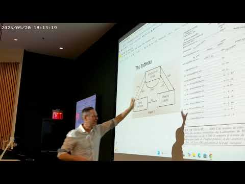
- François Quesnay, an 18th-century French physician and Louis XV’s personal doctor, modeled economic activity as flows among social classes.
- His Tableau Économique tracked exchanges between landowners, the productive class, and the sterile class.
- The example’s flows balance, reproducing a total of 600, and Baker notes its influence as an antecedent to Karl Marx’s class-based analysis.
- Modern macroeconomics generally groups economic participants as households and firms instead.
- In Baker’s simple economy, a worker earns wages at a flour mill, the mill supplies a bagel shop, and the worker spends wages on bagels.
- Tracking wages and bagel sales over a period offers a basic way to measure the economy’s activity.
- The example illustrates how the same production process generates both goods and income.
- Households supply land, labor, capital, and entrepreneurship to firms through factor markets.
- Firms combine these inputs to produce goods and services, which they sell in goods markets.
- Capital is ultimately owned by households; banks often act as financial intermediaries connecting household savings to firms.
- Firms pay wages, interest income, and profits, which become household income and return to firms as consumer spending.
- Government enters the circular flow by collecting taxes, making transfer payments, and purchasing goods and services.
- Examples of transfers include Social Security, welfare, unemployment insurance, and pandemic-era Paycheck Protection Program payments.
- For 2023, Baker cites government spending of about $6.1 trillion and tax collections of about $4.4 trillion.
- Government purchases include services such as hiring teachers, as well as buying goods and services from the private sector.
- Because an economy produces unlike items such as cars, apples, and oranges, their quantities cannot be meaningfully added without a common unit.
- GDP measures the dollar value of production, much as Costco’s roughly $303 billion in annual revenue aggregates sales across many product types.
- Baker notes Costco also paid about $290 billion for wages, suppliers, transport, and other costs, illustrating how firm revenue becomes income elsewhere.
- National output can be measured through spending on final goods, factor payments such as wages and profits, or value added; the measures should reconcile.
- Nominal values are face-value dollar amounts, while real values account for purchasing power.
- A Kentucky Fried Chicken meal in Iceland costing 3,249 Icelandic krónur is about $26, making its expense easier to assess against U.S. prices.
- The same adjustment is needed to judge whether a $400 car in 1932 was expensive relative to what money could buy then.
- A fixed bundle of goods, such as groceries, can help compare overall costs across years.
- Nominal U.S. GDP rises from about $244 billion in 1947 to roughly $32 trillion in the lecture’s present-day data.
- That increase overstates real production growth because the dollar’s purchasing power has declined as prices rose.
- The Consumer Price Index rises from 21 in February 1947 to about 337 in the contemporary series, implying prices roughly 12 to 13 times higher.
- Recession periods appear as gray bars on the GDP chart, with output growth flattening or reversing during economic slowdowns.
- Real GDP holds prices constant, removing price changes from comparisons of production over time.
- Using 2017 prices, Baker reports real GDP per capita rising from about $15,248 in 1947 to roughly $71,000 today.
- U.S. population grew from about 180 million in 1960 to 341 million, so total output alone does not show how much production is available per person.
- A long-run graph from 1871 to 2008 shows substantial real GDP per capita growth, alongside major disruptions such as the Great Depression and World War II.
- The example economy produces food, clothing, shelter, and transit, with each good measured in different units.
- Year one quantities are 20, 20, 30, and 15; multiplying them by prices of $4, $5, $8, and $2 gives nominal GDP of $450.
- Year two quantities are 22, 25, 32, and 20, with prices of $5, $6, $10, and $3; nominal GDP totals $640.
- The nominal increase combines changes in quantities with increases in prices, so it cannot isolate production growth.
- To calculate real GDP, Baker holds year-one prices fixed and applies them to each year’s quantities.
- Year one real GDP is $450, and year two real GDP is $509 using prices of $4, $5, $8, and $2.
- The increase from $450 to $509 reflects changed quantities rather than the rise in prices.
- The base year supplies the common price yardstick; the historical series shown earlier uses 2017 prices.
- Holding year-one quantities fixed while applying year-two prices raises the basket’s cost from $450 to $565, isolating price changes.
- The example contrasts two calculations: fixed prices with changing quantities measure real GDP, while fixed quantities with changing prices provide an inflation measure.
- Baker identifies inflation, interest rates, and real GDP growth as key rates of change used in macroeconomics.
- An account growing from $100 to $120 over a year earns a 20% interest rate, which is the money’s percentage growth over that period.
Transcript excerpt
0:00 Okay, here we go. Lecture 18. Uh kind of an exciting day where you can see we'll talk about introduction to macroeconomics today. Macroeconomics. Uh so it's a pretty uh you'll see it's a shift in uh a pretty substantial change in what we're doing. A good shift in our focus here. So we do just have a new chapter of reading up there. Chapter 14. Actually, I put three up because now they're just kind of really quick uh small chapters each with a particular concept that will occupy us over the next couple of classes. Uh before we dive in, uh it should be the case uh that your exam scores are up on grade scope and you should be able to have a look at them and complain or check your grading. Um see if there's any mistakes, uh argue for points, all of that stuff.
0:50 Um, I I say curved exam grades, but that's I think they're just going to kind of go up as they are, but I'm going to put everything back up, you know, into a a bright space. Um, all of it should be up there over the next week and then you can get a good idea as to where you stand overall in the class. Um, just some other bookkeeping in terms of our dates. We are getting down to the to the end of the uh class here. So, I'm just looking. I like to do this in front of the class just cuz it's a, you know, make sure I have it right. Here's the exam schedule. I believe this is us here. And so, our last class is the 14th. And then, which is great. So, we can have the review on the 14th and then we'll
This is the start of the transcript. Save this video free for the whole transcript, searchable and time-coded.
In this course
Related notes
Summary, takeaways, and chapters were generated by AI from the video's transcript and may contain errors. The video belongs to its creator, Matthew Baker.